Overview
The goal of this notebook is to review deep learning methods for object detection and image segmentation.
Performance Metrics
Let’s start with how the performance of image segmentation / object recognition is evaluated.
Reference: https://towardsdatascience.com/breaking-down-mean-average-precision-map-ae462f623a52
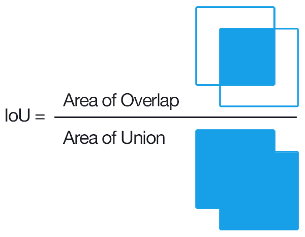
Intersection over Union (IoU)
IoU is given by the ratio of the area of intersection and area of union of the predicted bounding box and ground truth bounding box.
IoU can be used to determine if the bounding box is a case of true positive (TP), false positive (FP), or false negative (FN). IoU does not determine true negative, since we assume the ground truth bounding box contains an object (in another word, if it is a case of true negative, then the ground truth box contains no object).
Before we separate the 3 cases, we need to pre-determine a threshold (this is a hyperparameter). Much like logistic regression, a typical choice of threshold is 0.5 (however, in the original R-CNN paper, the threshold was set to 0.3, determined using a grid search over [0.0, 0.1, 0.2, 0.3, 0.4, 0.5]; of course, one may choose to optimize the threshold through ROC curves or some other diagnostic metrics like F1 score).
- True positive: If IoU > 0.5 and the label is correct, then we say the bounding box is a case of true positive (TP).
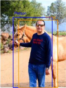
- False negative: If IoU > 0.5 but classify the wrong label, then we say the bounding box is a case of false negative (FN). For example, in the image below, the bounding box classify the person as horse
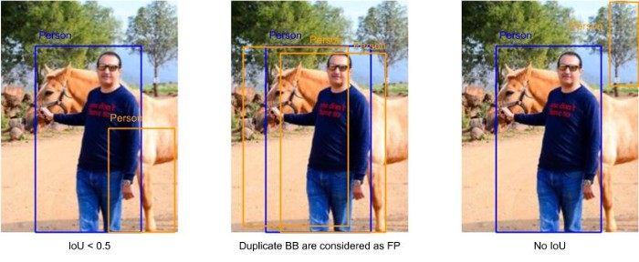
- False positive: There are 3 cases when a bounding box is determined as a false positive case (FP), illustrated in the following image
- IoU < 0.5
- No IoU (IoU = 0) (this can be used as a negative case)
- Duplicated bounding box (two bounding boxes that classify the same object)
Mean Average Precision (mAP)
The SVM classifier is binary and individually trained for each class. To assess the performance for all classes, we average the performance for each individual class.
Remember that in binary classification, there are several important metrics to determine performance of our model. One is by using precision-recall curve (as opposed to ROC curve). Specifically,
$\text{Precision} = \frac{\text{True Positives}}{\text{Predicted Positives}} = \frac{TP}{TP + FP}$
$\text{Recall} = \frac{\text{True Positives}}{\text{Actual Positives}} = \frac{TP}{TP + FN}$
We know there is a trade-off between precision and recall: as recall increases, precision decreases. Then the Average Precision metric will give an estimate on how the model performs (this is very much like a summary metric like AUC for ROC curves). To calculate Average Precision for each class,
- Divide the recall (let’s denote by $R$) between 0 and 1, into 11 intervals, i.e. [0, 0.1, …, 1.0]
- Given a recall level, we can calcualte the IoU threshold needed
- After calculating the IoU threshold, we can then find the corresponding precision (let’s denote it by $P$) that matched each level of recall. An example precision-recall curve is shown below:
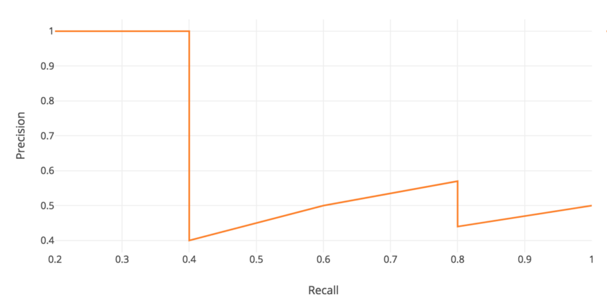
-
The precision-recall curve would usually look like a zig-zag. It may be better to “smooth” it. One way to do so is that, for each recall level $R$, replace the precision value at the current recall with the maximum precision value at recall levels greater than the current level (i.e. $>R$).
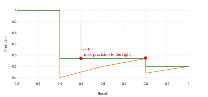
-
Then Average Precision is the average of the smoothed precisions (let’s denote the smoothed version with $\tilde{P}$), i.e. for the $i$-th class,
- However, later studies used the AUC metric after smoothing, instead of simply the average of the precisions, probably to account for the effect of recall more directly. Also, instead of sampling only 11 points, it samples more points. There are several variants of ways to calculate AP.
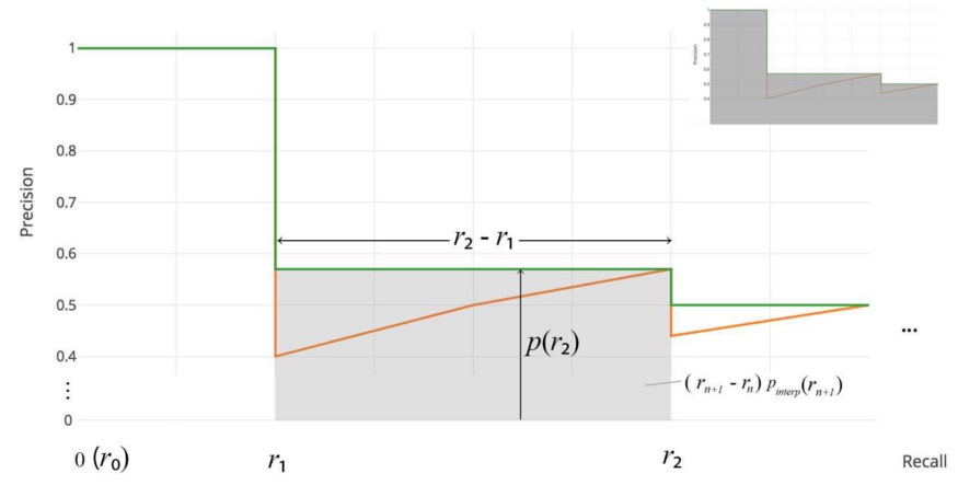
- Lastly, the mAP is calcualted as the average of Average Precision over all $N$ classes, i.e.
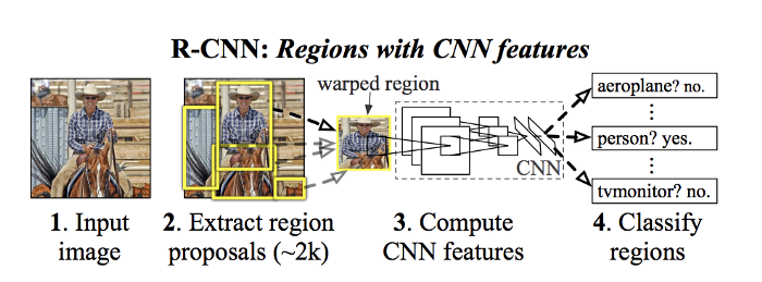
R-CNN
Model Workflow
The algorithm proceeds with the following steps:
- Use Selective Search to propose about 2000 regions (bounding boxes)
- For each proposed regions, warp the image within the bounding box into a $227 \times 227$ image
- Run the warped images through a pre-trained AlexNet to extract features of the image
- 5 convolutional layers and 2 fully connected layers
- Resulting a feature vector of 4096 in length
- Feed the extracted features to SVM to classify the presence of the object
- For each class of object, they train a binary SVM classifier
- Run the bonuding box through a linear regression model to output tighter coordinates for the box once the object has been classified.
Notice that 3 different models were involved: 1) CNN, 2) SVM, and 3) Linear regression.
Selective Search
References:
https://www.learnopencv.com/selective-search-for-object-detection-cpp-python/
Selective Search for Object Recognition
Selective search is a region proposal algorithm. An advantage of region proposal algorithm is that it has high recall, i.e. capturing more positive cases. This, in turn, would also mean there will be a lot of false positives, where proposed region does not contain target object. It sacrafices false positives in exchange for reducing false negatives.
Broadly, selective search starts with over-segmented images. Then group those segments by their 4 measures of similarity, i.e. color, texture, size, and shape compatibility. Selective search uses the following steps repeatedly:
- Add all bounding boxes corresponding to segmented parts to the list of regional proposals
- Group adjacent segments based on similarity
- Go to step 1
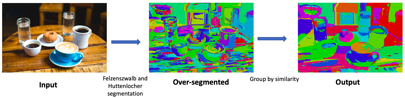
Smaller segments are combined into larger segments iteration by iteration. This is why building of the proposed regions is said to be “hierarchical”
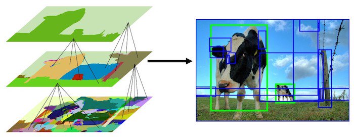
Similarity
Color
For each region $r_i$, calculate the color histogram of 25 bins for all 3 color channel, total 75 bins. Thus each region’s color profile can be represented by this vector of length 75. Then the color similarity between two proposed regions $r_i$, and $r_j$ is calcualted as
where $c_i^{(k)}$, $c_j^{(k)}$ is the height of $k$-th bin in the color descriptor for proposed region $r_i$ and $r_j$, respectively.
Texture
For each color channel, and each of 8 directions (8 neighbors, i.e. up, down, left, right, lower-left, upper-left, lower-right, upper-right), take Gaussian Derivative (i.e. convolve the image with a Gaussian kernel’s derivative taken in 8 directions, see https://cw.fel.cvut.cz/old/_media/courses/ucuws17/gd.pdf), with Gaussian kernel of size $\sigma=1$.
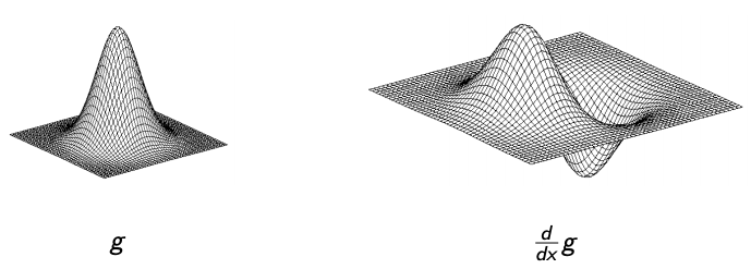
For each resulting image (total $3 \times 8 = 24$ images), construct a histogram with 10 bins. This results a texture feature vector of length 240. Then, the similarity in texture is calcualted as
where $t_i^{(n)}$, $t_j^{(n)}$ is the height of $n$-th bin in the texture descriptor for proposed region $r_i$ and $r_j$, respectively.
Size
Size similarity encourages smaller regions to merge first. It is defined as the fraction of image that $r_i$ and $r_j$ jointly occupy.
where $\text{size}(r_i)$, $\text{size}(r_j)$, and $\text{size}(image)$ are sizes of proposed regions $r_i$, $r_j$ and size of input image in number of pixels, respectively.
Shape compatibility
Shape compatilbity measures how $r_i$ fits with $r_j$. If $r_i$ fits $r_j$, then we should merge them, and fill any gaps in between. If they are not even touching each other, then they should not be filled.
Final similarity
where $a_n \in 0, 1$ to indicate whether the similarity measure is used or not.
Objectness
Reference http://groups.inf.ed.ac.uk/calvin/objectness/
Measuring the objectness of image windows
The resulting proposed regions are sorted in Objectness. It quantifies how likely it is for an image window to contain an object of any class, such as cars and dogs, as opposed to backgrounds, such as grass and water.
The objectiveness model is built based on Naive Bayses, and trained using features such as color contrasts, closed form of the edges of an object, edge characteristics, etc. to estimate the probability of an proposed window contains an object.
Example Use of Selective Search in Python OpenCV
#!/usr/bin/env python
'''
Usage:
    ./ssearch.py input_image (f|q)
    f=fast, q=quality
Use "l" to display less rects, 'm' to display more rects, "q" to quit.
'''

import sys
import cv2

if __name__ == '__main__':
    # If image path and f/q is not passed as command
    # line arguments, quit and display help message
    if len(sys.argv) < 3:
        print(__doc__)
        sys.exit(1)

    # speed-up using multithreads
    cv2.setUseOptimized(True);
    cv2.setNumThreads(4);

    # read image
    im = cv2.imread(sys.argv[1])
    # resize image
    newHeight = 200
    newWidth = int(im.shape[1]*200/im.shape[0])
    im = cv2.resize(im, (newWidth, newHeight))

    # create Selective Search Segmentation Object using default parameters
    ss = cv2.ximgproc.segmentation.createSelectiveSearchSegmentation()

    # set input image on which we will run segmentation
    ss.setBaseImage(im)

    # Switch to fast but low recall Selective Search method
    if (sys.argv[2] == 'f'):
        ss.switchToSelectiveSearchFast()

    # Switch to high recall but slow Selective Search method
    elif (sys.argv[2] == 'q'):
        ss.switchToSelectiveSearchQuality()
    # if argument is neither f nor q print help message
    else:
        print(__doc__)
        sys.exit(1)

    # run selective search segmentation on input image
    rects = ss.process()
    print('Total Number of Region Proposals: {}'.format(len(rects)))

    # number of region proposals to show
    numShowRects = 100
    # increment to increase/decrease total number
    # of reason proposals to be shown
    increment = 50

    while True:
        # create a copy of original image
        imOut = im.copy()

        # itereate over all the region proposals
        for i, rect in enumerate(rects):
            # draw rectangle for region proposal till numShowRects
            if (i < numShowRects):
                x, y, w, h = rect
                cv2.rectangle(imOut, (x, y), (x+w, y+h), (0, 255, 0), 1, cv2.LINE_AA)
            else:
                break

        # show output
        cv2.imshow("Output", imOut)

        # record key press
        k = cv2.waitKey(0) & 0xFF

        # m is pressed
        if k == 109:
            # increase total number of rectangles to show by increment
            numShowRects += increment
        # l is pressed
        elif k == 108 and numShowRects > increment:
            # decrease total number of rectangles to show by increment
            numShowRects -= increment
        # q is pressed
        elif k == 113:
            break
    # close image show window
    cv2.destroyAllWindows()
Tightening bounding box
Given a region proposal $\mathbf{p} = {p_x, p_y, p_w, p_h }$, and ground truth $\mathbf{g} = { g_x, g_y, g_w, g_h }$ (both specified in the format of a bounding box: $x$ coordinate, $y$ coordinate, width, and height), we can transform the proposed region $\mathbf{p}$ into predicted ground truth $\hat{\mathbf{g}}$ by applying the following transformation
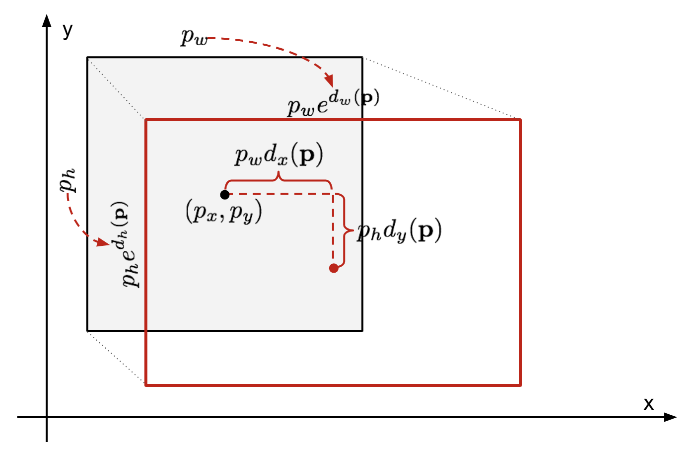
with transformation
where $\phi_5(\mathbf{p})$ is the feature transformation from pool5 layer of the AlexNet given proposed feature $\mathbf{p}$, with $* \in {x, y, w, h}$.
$\mathbf{w}_*$ is a learned parameter given by the following ridge regression
with $i$ as the index of the proposal and $N$ as the total number of proposal. The target $t_*$ is specified as
which are simply the reverse transformation for $\hat{g}_*$. $\lambda:=1000$ based on validation.
Additional Tricks
Verbatim copy from: https://lilianweng.github.io/lil-log/2017/12/31/object-recognition-for-dummies-part-3.html
Note that these additional tricks dealt with false positives. They reduce duplicate detection using Non-Maximum Suppression, and take advantage of $IoU<0.5$ with Hard Negative Mining to improve SVM classification ($IoU = 0$ would be an Easy Negative by contrast).
Hard Negative Mining
We consider bounding boxes without objects as negative examples. Not all the negative examples are equally hard to be identified. For example, if it holds pure empty background, it is likely an “easy negative”; but if the box contains weird noisy texture or partial object, it could be hard to be recognized and these are “hard negative”.
The hard negative examples are easily misclassified. We can explicitly find those false positive samples during the training loops and include them in the training data so as to improve the classifier.
Non-Maximum Suppression (NMS)
Likely the model is able to find multiple bounding boxes for the same object. Non-max suppression helps avoid repeated detection of the same instance. After we get a set of matched bounding boxes for the same object category:
- Sort all the bounding boxes by confidence score.
- Discard boxes with low confidence scores.
- While there is any remaining bounding box, repeat the following:
- Greedily select the one with the highest score, commit to output
- Remove the boxes with high IoU (e.g. > 0.5) with this box with highest score (Then, go to find the bounding box with the next highest scores in the list of bounding boxes to commit to output, and remove others with high overlap / IoU with that box, …etc.)
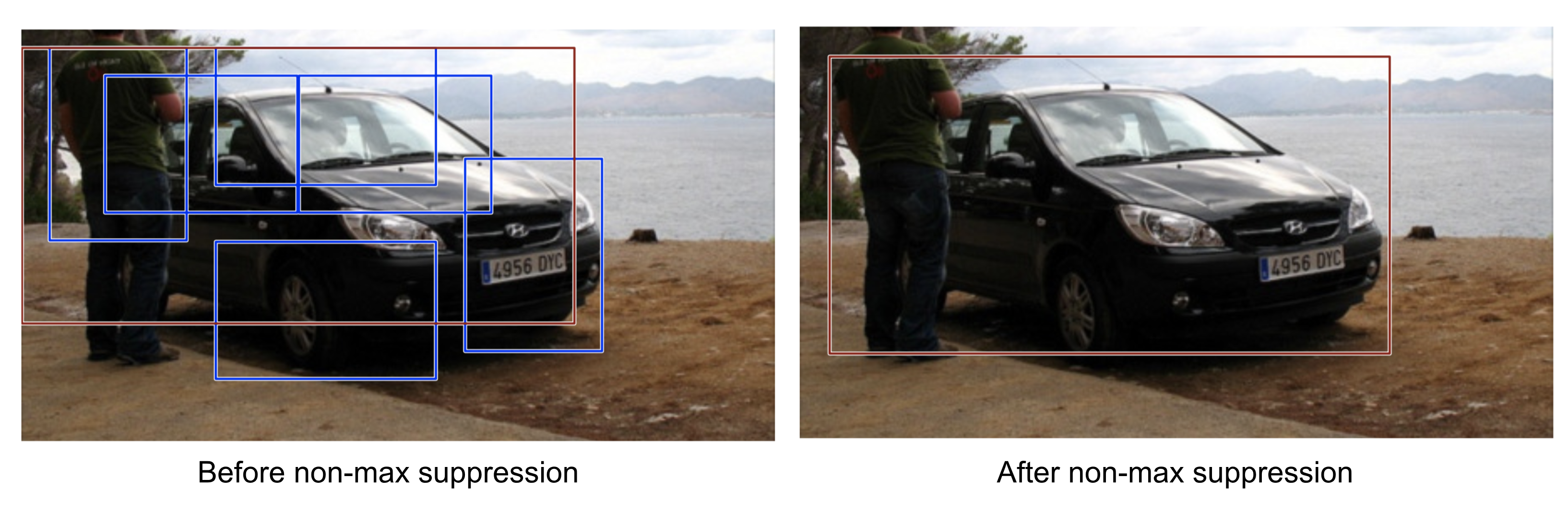
Multiple bounding boxes detect the car in the image. After non-maximum suppression, only the best remains and the rest are ignored as they have large overlaps with the selected one. (Image source: DPM paper)
Here is a Python implementation of NMS
import numpy as np

def nms(dets, thresh):
    x1 = dets[:, 0]
    y1 = dets[:, 1]
    x2 = dets[:, 2]
    y2 = dets[:, 3]
    scores = dets[:, 4]

    areas = (x2 - x1 + 1) * (y2 - y1 + 1)
    # Sort scores by descending order
    order = scores.argsort()[::-1]

    keep = []
    while order.size > 0:
        i = order[0]# index of highest score
        keep.append(i)
        xx1 = np.maximum(x1[i], x1[order[1:]])
        yy1 = np.maximum(y1[i], y1[order[1:]])
        xx2 = np.minimum(x2[i], x2[order[1:]])
        yy2 = np.minimum(y2[i], y2[order[1:]])

        w = np.maximum(0.0, xx2 - xx1 + 1)
        h = np.maximum(0.0, yy2 - yy1 + 1)
        inter = w * h # area of intersection
        ovr = inter / (areas[i] + areas[order[1:]] - inter) # IoU vectors

        inds = np.where(ovr <= thresh)[0]
        order = order[inds + 1]

    return keep
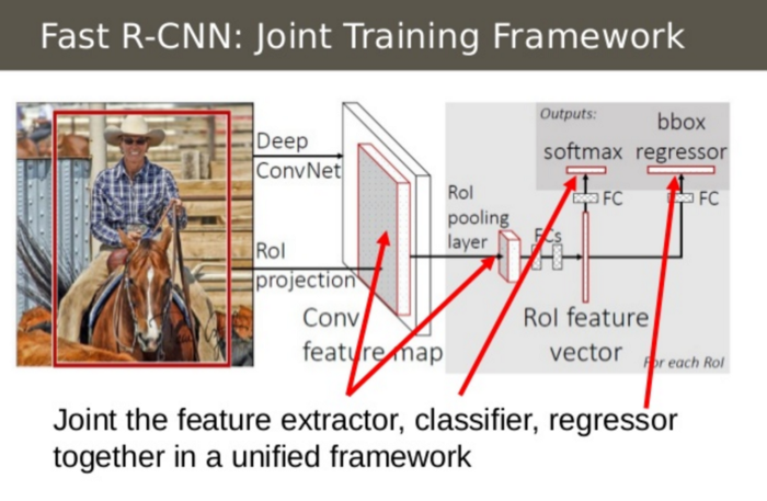
Fast R-CNN
Fast R-CNN integrates CNN feature extraction, classification, and linear regression of bounding boxes in the same framework, therefore, speeding up training and prediction significantly.
Model workflow
Reference: https://lilianweng.github.io/lil-log/2017/12/31/object-recognition-for-dummies-part-3.html
How Fast R-CNN works is summarized as follows; many steps are same as in R-CNN:
- First, pre-train a convolutional neural network on image classification tasks.
- Propose regions by selective search (~2k candidates per image).
- Alter the pre-trained CNN:
- Replace the last max pooling layer of the pre-trained CNN with a ROI pooling layer. The ROI pooling layer outputs fixed-length feature vectors of region proposals. Sharing the CNN computation makes a lot of sense, as many region proposals of the same images are highly overlapped.
- Replace the last fully connected layer and the last softmax layer (originally 1000 classes) with the following two branches in parallel
- Finally the model branches into two sibling output layers:
- A softmax estimator of K + 1 classes (same as in R-CNN, +1 is the “background” class), outputing a discrete probability distribution per ROI.
- A bounding-box regression model which predicts offsets relative to the original ROI for each of K classes.
ROI pooling
Reference: https://deepsense.ai/region-of-interest-pooling-explained/
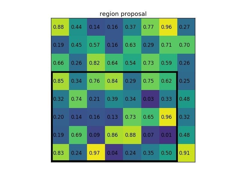
In the original R-CNN, forward pass of AlexNet was done on all ~2000 proposed regions, one by one. This slows down the network. The author therefore proposed ROI pooling. Instead of feeding each proposed region into the ConvNet, pass the original image, and then pool the extracted features based on the proposed regions. ROI pooling operates in the following steps:
- Given feature map (e.g. 8x8) from convolutional layers and a list of proposed regions ($N \times 5$ for $N$ proposed regions, where each row is [index, x, y, width, height])

-
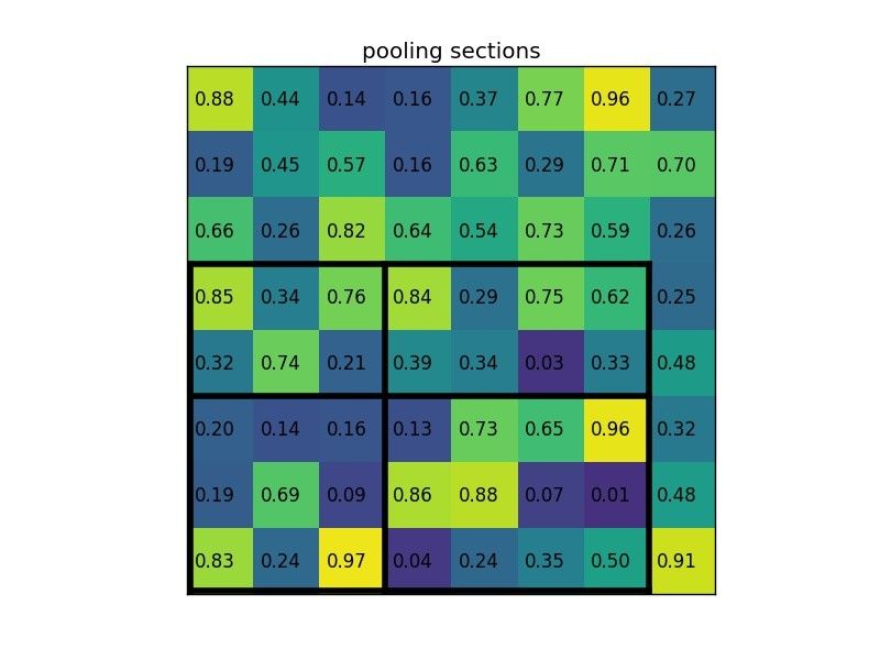
Divide the proposed regions into a pre-specified sub-regions (e.g. 2x2), each with equal size
-
Max pool to get 2x2 features for each proposed region
An animated walk-through of ROI pooling

- Stack the resulted ROI pooling features for each proposed region. This converts proposed regions of different sizes into a stack of features with the same step.
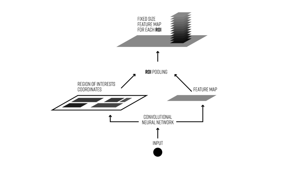
In summary, given an input image of size $W \times H \times 3$, and a list of proposed regions of length $N$. We extract ROI features of size $w \times h$ for all $N$ proposed regions, resulting a matrix of $w \times h \times N \times 3$.
Classification
Instead of training an SVM for each class, Fast R-CNN now uses a softmax layer to output the probability of each class.
Loss Function
Reference: Verbatim from https://lilianweng.github.io/lil-log/2017/12/31/object-recognition-for-dummies-part-3.html
The model is optimized for a loss combining two tasks (classification + localization via regression):
| Symbol | Explanation |
|---|---|
| $u$ | True class label, $u \in 0,1,…,K$; by convention, the catch-all background class has $u=0$. |
| $\mathbf{p}$ | Discrete probability distribution (per ROI) over $K + 1$ classes: $\mathbf{p}=(p_0,…,p_K)$, computed by a softmax over the $K + 1$ outputs of a fully connected layer. |
| $\mathbf{v}$ | True bounding box $\mathbf{v}=(v_x,v_y,v_w,v_h)$. |
| $\mathbf{t}^{(u)}$ | Predicted bounding box correction, $\mathbf{t}^{(u)}=(t^{(u)}_x,t^{(u)}_y,t^{(u)}_w,t^{(u)}_h)$. |
The loss function sums up the cost of classification and bounding box regression: $\mathcal{L} = \mathcal{L}_{cls}+\mathcal{L}_{reg}$. For “background” ROI, $\mathcal{L}_{reg}$ is ignored by the indicator function $\mathbb{1}[u > 1]$ defined as:
The overall loss function is:
The bounding box loss $\mathcal{L}_{reg}$ should measure the difference between $t^{(u)}_i$ and $v_i$ using a robust loss function. The smooth $L1$ loss is adopted here and it is claimed to be less sensitive to outliers.
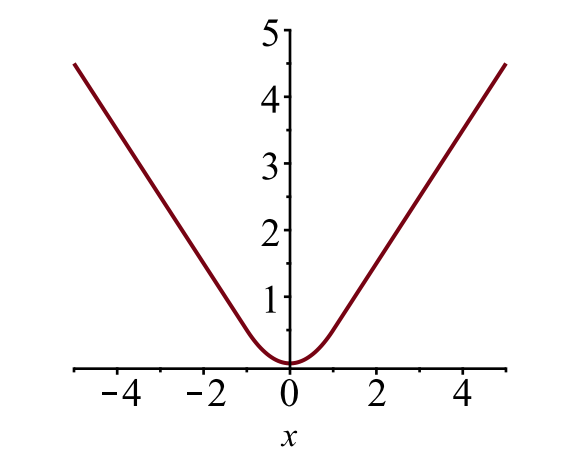
The plot of smooth $L1$ loss, $y=L^{smooth}_1(x)$. (Image source: link)
A word on backpropgation gradient on Max pooling and ROI pooling
Reference: https://datascience.stackexchange.com/questions/11699/backprop-through-max-pooling-layers
For max pooling, there is no gradient with respect to non maximum values, since changing them slightly does not affect the output. Further the max is locally linear with slope 1, with respect to the input that actually achieves the max. Thus, the gradient from the next layer is passed back to only that neuron which achieved the max. All other neurons get zero gradient.
So in your example, $\delta^{(l)}_i$ would be a vector of all zeros, except that the $i^∗$-th location will get a value ${ \delta^{(l+1)}_j }$ where
Similarly, for ROI pooling,
There is no gradient ($\delta_i^{(l)}=0$) except for the sub-region of the ROI that was max
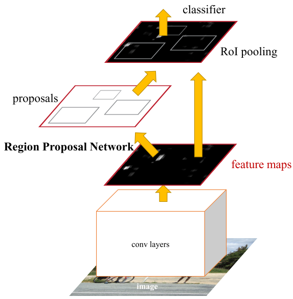
Faster R-CNN
Faster R-CNN now let region proposal network (RPN) and the Fast R-CNN network share the CNN features. Therefore, the entire network now learns to propose regions, which greatly speed up training and prediction.
Here is a brief description of Faster R-CNN, from the Mask R-CNN paper:
Faster R-CNN consists of two stages. The first stage, called a Region Proposal Network (RPN), proposes candidate object bounding boxes. The second stage, which is in essence Fast R-CNN [12], extracts features using RoIPool from each candidate box and performs classification and bounding-box regression. The features used by both stages can be shared for faster inference.
Model Workflow
- Pre-train a CNN network on image classification tasks.
- Fine-tune the RPN (region proposal network) end-to-end for the region proposal task, which is initialized by the pre-trained image classifier. Positive samples have IoU (intersection-over-union) > 0.7, while negative samples have IoU < 0.3.
- Slide a small $n \times n$ spatial window over the conv feature map of the entire image.
- At the center of each sliding window, we predict multiple regions of various scales and ratios simultaneously. An anchor is a combination of (sliding window center, scale, ratio). For example, 3 scales + 3 ratios => k=9 anchors at each sliding position.
- Train a Fast R-CNN object detection model using the proposals generated by the current RPN
- Then use the Fast R-CNN network to initialize RPN training. While keeping the shared convolutional layers, only fine-tune the RPN-specific layers. At this stage, RPN and the detection network have shared convolutional layers!
- Finally fine-tune the unique layers of Fast R-CNN
- Step 4-5 can be repeated to train RPN and Fast R-CNN alternatively if needed.
Region Proposal Networks (RPN)
A Region Proposal Network (RPN) takes an image (of any size) as input and outputs a set of rectangular object proposals, each with an objectness score. The output of a region proposal network (RPN) is a bunch of boxes/proposals that will be examined by a classifier and regressor to eventually check the occurrence of objects. To be more precise, RPN predicts the possibility of an anchor being background or foreground, and refine the anchor.
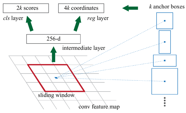
An RPN is implemented as two convolutional layers: a convolutional layer with kernel size of $n \times n$ ($n=3$ in the original paper), followed by two sibiling convolutional layers with kernel size $1 \times 1$ (one for $reg$ and one for $cls$, respectively)
The input of the RPN (i.e. for the first $n \times n$ convolutional layer) is a feature map (of size $w \times h$) output from either ZF (filter dimension 256) or VGG (filter dimension 512) network. The $n \times n$ convolutional layer uses stride of 1 and padding of 1. Thus, the ouptut of this $n \times n$ is $w \times h \times 256$ or $w \times h \times 512$.
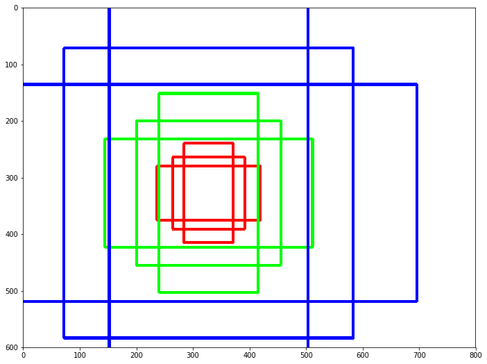
For each pixel in the feature map, we choose variations in 3 aspect ratios and 3 scales, which we call anchors of that pixel. Therefore, there are total $k=9$ anchors for each pixel. The type of anchors are: $(128^2, 256^2, 512^2) \times ([1, 1], [1,2], [2,1])$. The following figure shows all 9 anchors in a $800 \times 600$ image.
Thus, for all the pixels, we have $k \times w \times h = 9 \times 40 \times 60 = 21600$ anchors. We ignore the anchors that bleed beyond the borders of the image, which left us with ~6000 validanchors. Then we apply NMS and this leaves us with about 2000 anchors
We further divide the proposed regions into 3 categories
- IoU > 0.7: is object (positive anchors)
- 0.3 < IoU < 0.7: ambiguous (neutral anchors)
- IoU < 0.3: not object (negative anchors)
For each mini-batch (from a single image) during training, we randomly sample 128 positive anchors and 128 negative anchors. Because most of the anchors are negative anchors, random sampling of anchors helps balance the number of positive and negative anchors.
The two outputs of the RPN (i.e. outupt of $1 \times 1$ convolutional layer) vary in size, depending on the classification or regression task.
Recall that $1 \times 1$ convolution is a technique used to change filter dimensions. Classification requires 2 neurons to encode whether a proposal is or is not an object (logit representation of background / foreground; of course, with a single sigmoid activation, the probability only need to be encoded with 1 neuron; but 2 is the choice of the original paper). Regression requires 4 neurons to encode the 4 parameters of the bounding box ($x, y, w, h$). We need to encode these parameters for each of $k=9$ anchors. Therefore, we need to output $2k=2 \times 9 = 18$ channels for $cls$ layer and $4k = 4 \times 9 = 36$ channels for $reg$ layer.
Note that the labels we need to create before we start training the network also needs to be in the same dimensions ($w \times h \times 2k$ and $w \times h \times 4k$, respectively), since our data for the classifier and regressor are simply a batch of proposed bounding boxes. Also, We don’t actually need to extract image region within the proposed anchors (to determine labels, we just need to calcualte the anchor projected in the input image based on the receptive field, i.e. given a neuron / pixel in the CNN feature, what is the original center of the receptive field of this neuron; from that center of that neuron, we can draw 9 anchors). The proposed regions are simply being input into the regressor and classifier to compare against the ground truth bounding boxes (see the loss function below).
Loss Function
Faster R-CNN is optimized for a multi-task loss function, similar to fast R-CNN.
| Symbol | Explanation |
|---|---|
| $p_i$ | Predicted probability of anchor $i$ being an object. |
| $p^∗_i$ | Ground truth label (binary) of whether anchor $i$ is an object. |
| $\mathbf{t}_i$ | A vector of predicted four parameterized coordinates for anchor $i$. |
| $\mathbf{t}^∗_i$ | A vector of ground truth coordinates for anchor $i$. |
| $N_{cls}$ | Normalization term, set to be mini-batch size (~256) in the paper. |
| $N_{reg}$ | Normalization term, set to the number of anchor locations (~2400) in the paper. |
| $\lambda$ | A balancing parameter, set to be ~10 in the paper (so that both $\mathcal{L}_{cls}$ and $\mathcal{L}_{box}$ terms are roughly equally weighted). |
The multi-task loss function combines the losses of classification and bounding box regression:
where $i$ is the index of an anchor in a mini-batch, and $\mathcal{L}_{cls}$ is the log loss function over two classes,
as we can easily translate a multi-class classification into a binary classification by predicting a sample being a target object versus not. $L_1^{smooth}$ is the smooth $L_1$ loss.
Mask R-CNN
Reference: https://lilianweng.github.io/lil-log/2017/12/31/object-recognition-for-dummies-part-3.html#bounding-box-regression
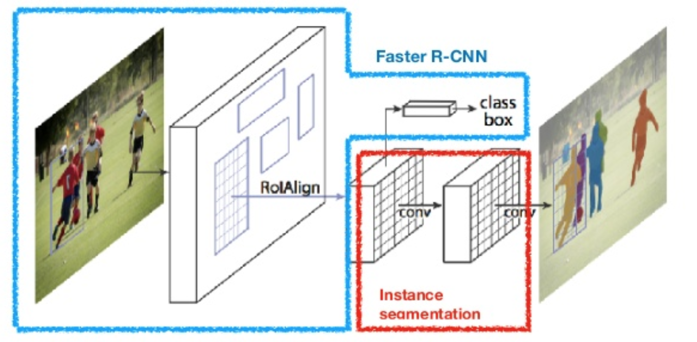
Mask R-CNN add a 3rd convolutional branch that does pixel-wise segmentation.
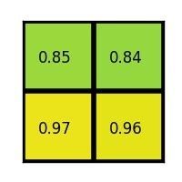
Mask labels
Ground truth mask is simply a label on each pixel of the original image.
More generally, an image is parcellated into grids (called cells). Each grid is then labeled. In Mask R-CNN, the mask is always parcellated into $m \times m$ grids for each of total $K$ classes, therefore, a total $K \times m \times m$ dimension label for each ROI. This is also the dimension of the output of the mask branch.
ROIAlign
Reference: https://blog.athelas.com/a-brief-history-of-cnns-in-image-segmentation-from-r-cnn-to-mask-r-cnn-34ea83205de4
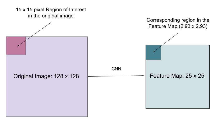
ROIAlign is a more accurate variant of ROI pooling. Suppose we have an input image of $128 \times 128$ and a feature mape of $25 \times 25$. A $15 \times 15$ ROI in the original image should scale down to $15 \times (25 / 128) \approx 2.93 \times 2.93$ ROI in the feature map. In ROI pooling, we would round this down to $2 \times 2$. Therefore, the alignment between the original image and ROI in the feature map projected back to the original image is mis-aligned.
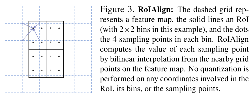
Instead of rounding down, ROIalign uses bilinear interpolation to estimate what a $2.93 \times 2.93$ ROI would be like, and pool that interpolated ROI in the feautre map.
Original paper’s explanation
Loss function
Since there are 3 branches now, the total loss is then
where the $\mathcal{L}_{cls}$ and $\mathcal{L}_{reg}$ are the same as Faster R-CNN, still classifying and regressing bounding boxes.
$\mathcal{L}_{mask}$ is defined as the average binary cross-entropy loss, only including $k$-th mask if the region is associated with the ground truth class $k$.
where $y_{ij}$ is the label of a cell $(i, j)$ in the true mask for the region of size $m \times m$; $\hat{y}^k_{ij}$ is the predicted value of the same cell in the mask learned for the ground-truth class $k$.
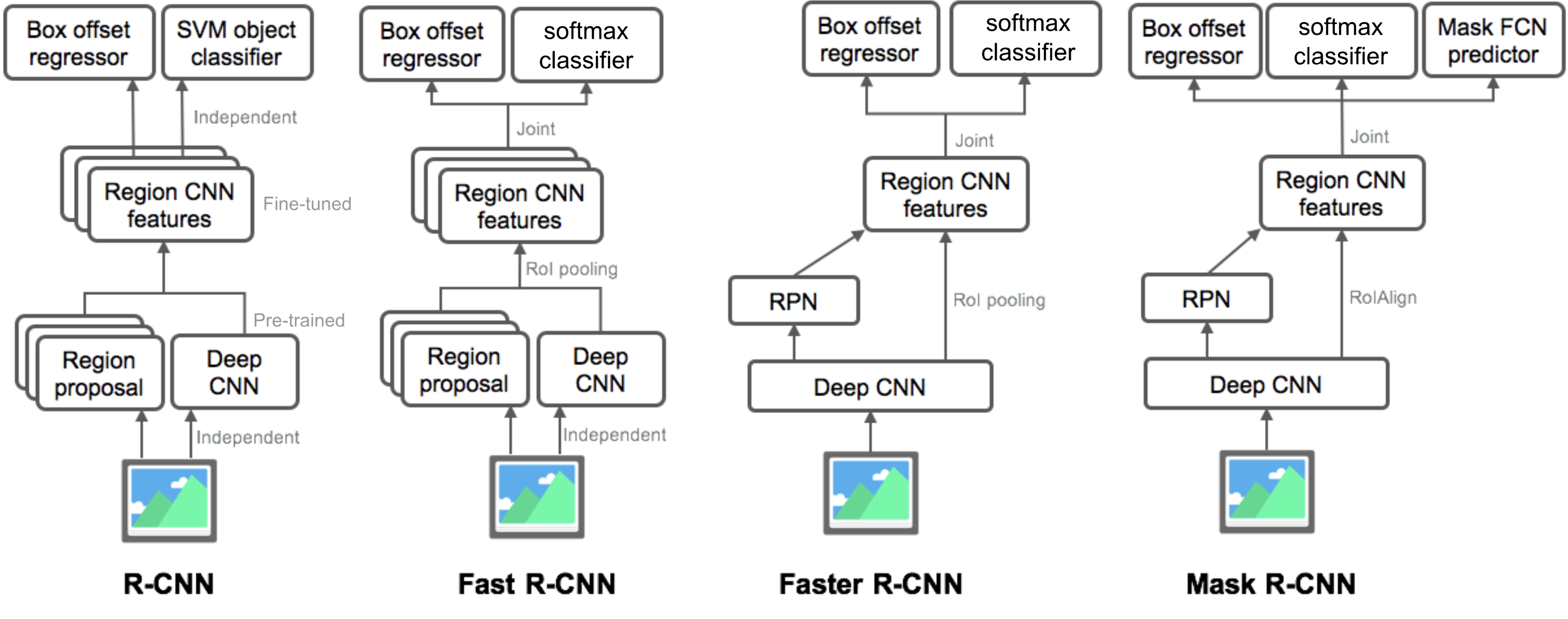
Comparison of R-CNN frameworks
Summary of Architecture
Reference: https://lilianweng.github.io/lil-log/2017/12/31/object-recognition-for-dummies-part-3.html#bounding-box-regression
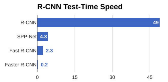
Performance at test-time, value in seconds.
Reference: https://towardsdatascience.com/r-cnn-fast-r-cnn-faster-r-cnn-yolo-object-detection-algorithms-36d53571365e