From DeepFake to Generative Adversarial Network (GAN)

We briefly review recent advancement in DeepFake research (e.g. face swapping).

DeepFake

Reference: https://www.kdnuggets.com/2018/03/exploring-deepfakes.html/2

The basic idea is to train 2 auto-encoders.

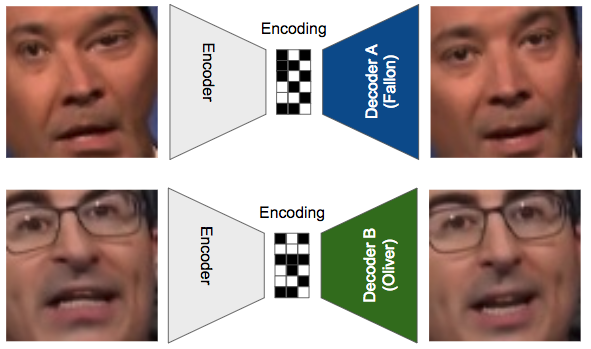
We pass in a warped image of Fallon to the encoder and try to reconstruct Fallon’s face with Decoder A. This forces Decoder A to learn how to create Fallon’s face from a noisy input.
Then, using the same encoder, we encode a warped version of Oliver’s face and try to reconstruct it using Decoder B.
We keep doing this over and over again until the two decoders can create their respective faces, and the encoder has learned how to “capture the essence of a face” whether it be Fallon’s or Oliver’s.

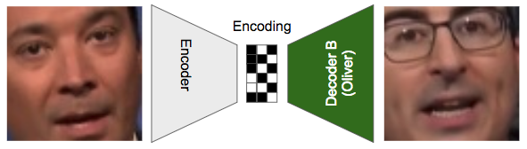
Pass in an image of Fallon into the encoder, and then instead of trying to reconstruct Fallon from the encoding, we now pass it to Decoder B to reconstruct Oliver.

Generative Adversarial Network (GAN)

Original paper: https://papers.nips.cc/paper/5423-generative-adversarial-nets.pdf

Consider a criminal trying to make counterfeit money, while police is trying to detect the fake money. The criminal tries the best to make the fake money as real as possible, while the police punishes the criminal when detecting the fake money.

The criminal making the fake money is called the Generator (denoted by $G$), and the police for detecting fake money and punishing the criminal is called the Discriminator (denoted by $D$).

Cost-function of GAN model:

$\begin{align}\mathcal{L}_D^{GAN} &= \mathbb{E}(\log D(x)) + \mathbb{E}(1 - \log( D(G(z)))\\ \mathcal{L}_G^{GAN} &= \mathbb{E}(\log( D(G(z))) \end{align}$

In lay terms, the discriminator wants to maximize the accuracy to correctly classify the real images as real, plus correctly classify the fake images as fake (or minimize incorrectly classify fake images as real).

The generator, on the other hand, want the discriminator to classify the generated images as real as much as possible.

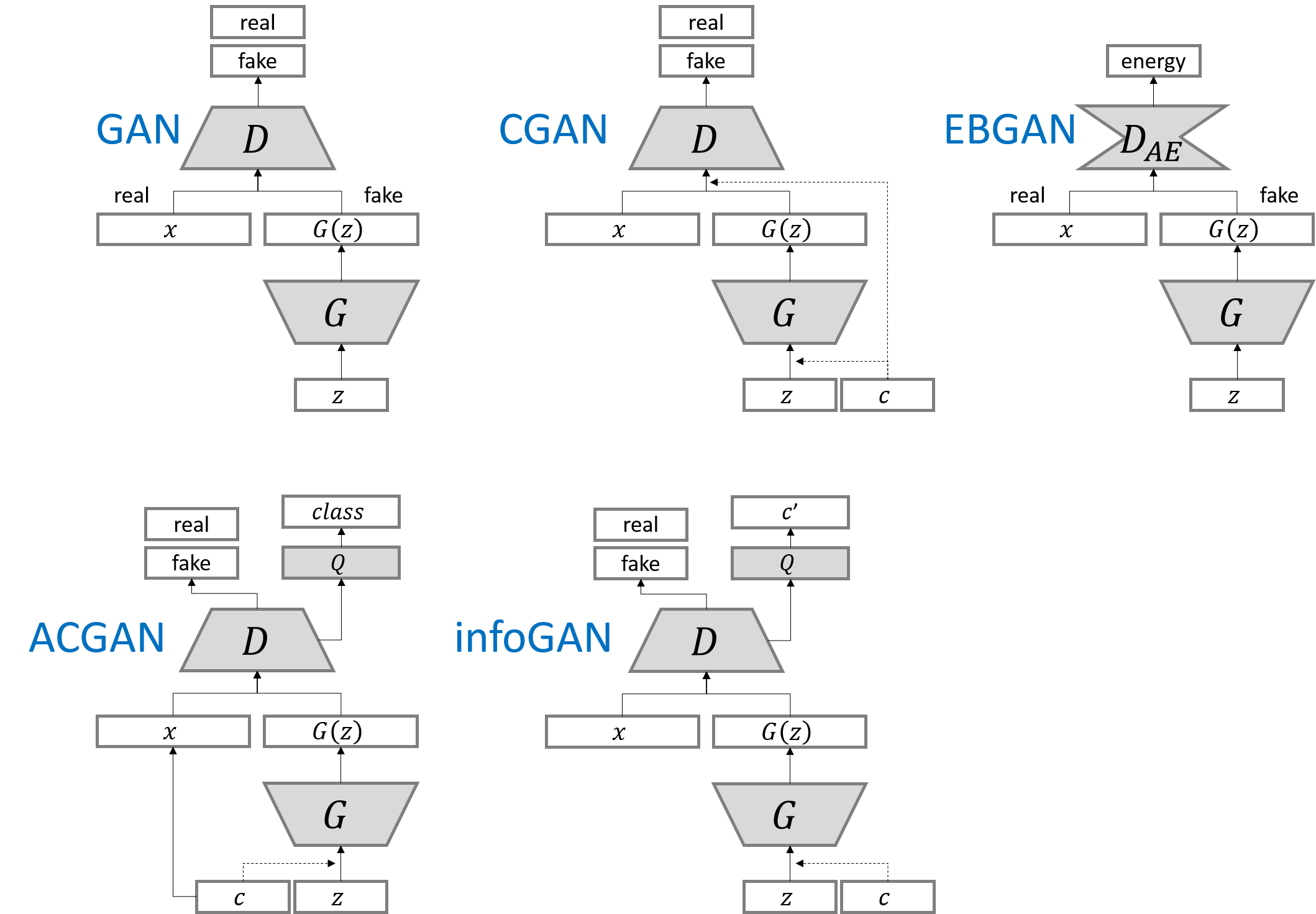
And some variants of the GAN structures

Implementation of Vanilla GAN using Keras

eriklindernoren/Keras-GAN

Training on MNIST dataset

class GAN():
    def __init__(self):
        self.img_rows = 28
        self.img_cols = 28
        self.channels = 1
        self.img_shape = (self.img_rows, self.img_cols, self.channels)

        optimizer = Adam(0.0002, 0.5)

        # Build and compile the discriminator
        self.discriminator = self.build_discriminator()
        self.discriminator.compile(loss='binary_crossentropy',
            optimizer=optimizer,
            metrics=['accuracy'])

        # Build and compile the generator
        self.generator = self.build_generator()
        self.generator.compile(loss='binary_crossentropy', optimizer=optimizer)

        # The generator takes noise as input and generated imgs
        z = Input(shape=(100,))
        img = self.generator(z)

        # For the combined model we will only train the generator
        self.discriminator.trainable = False

        # The valid takes generated images as input and determines validity
        valid = self.discriminator(img)

        # The combined model  (stacked generator and discriminator) takes
        # noise as input => generates images => determines validity
        self.combined = Model(z, valid)
        self.combined.compile(loss='binary_crossentropy', optimizer=optimizer)

    def build_generator(self):

        noise_shape = (100,)

        model = Sequential()

        model.add(Dense(256, input_shape=noise_shape))
        model.add(LeakyReLU(alpha=0.2))
        model.add(BatchNormalization(momentum=0.8))
        model.add(Dense(512))
        model.add(LeakyReLU(alpha=0.2))
        model.add(BatchNormalization(momentum=0.8))
        model.add(Dense(1024))
        model.add(LeakyReLU(alpha=0.2))
        model.add(BatchNormalization(momentum=0.8))
        model.add(Dense(np.prod(self.img_shape), activation='tanh'))
        model.add(Reshape(self.img_shape))

        model.summary()

        noise = Input(shape=noise_shape)
        img = model(noise)

        return Model(noise, img)

    def build_discriminator(self):

        img_shape = (self.img_rows, self.img_cols, self.channels)

        model = Sequential()

        model.add(Flatten(input_shape=img_shape))
        model.add(Dense(512))
        model.add(LeakyReLU(alpha=0.2))
        model.add(Dense(256))
        model.add(LeakyReLU(alpha=0.2))
        model.add(Dense(1, activation='sigmoid'))
        model.summary()

        img = Input(shape=img_shape)
        validity = model(img)

        return Model(img, validity)

    def train(self, epochs, batch_size=128, save_interval=50):

        # Load the dataset
        (X_train, _), (_, _) = mnist.load_data()

        # Rescale -1 to 1
        X_train = (X_train.astype(np.float32) - 127.5) / 127.5
        X_train = np.expand_dims(X_train, axis=3)

        half_batch = int(batch_size / 2)

        for epoch in range(epochs):

            # ---------------------
            #  Train Discriminator
            # ---------------------

            # Select a random half batch of images
            idx = np.random.randint(0, X_train.shape[0], half_batch)
            imgs = X_train[idx]

            noise = np.random.normal(0, 1, (half_batch, 100))

            # Generate a half batch of new images
            gen_imgs = self.generator.predict(noise)

            # Train the discriminator
            d_loss_real = self.discriminator.train_on_batch(imgs, np.ones((half_batch, 1)))
            d_loss_fake = self.discriminator.train_on_batch(gen_imgs, np.zeros((half_batch, 1)))
            d_loss = 0.5 * np.add(d_loss_real, d_loss_fake)


            # ---------------------
            #  Train Generator
            # ---------------------

            noise = np.random.normal(0, 1, (batch_size, 100))

            # The generator wants the discriminator to label the generated samples
            # as valid (ones)
            valid_y = np.array([1] * batch_size)

            # Train the generator
            g_loss = self.combined.train_on_batch(noise, valid_y)

            # Plot the progress
            print ("%d [D loss: %f, acc.: %.2f%%] [G loss: %f]" % (epoch, d_loss[0], 100*d_loss[1], g_loss))

            # If at save interval => save generated image samples
            if epoch % save_interval == 0:
                self.save_imgs(epoch)

    def save_imgs(self, epoch):
        r, c = 5, 5
        noise = np.random.normal(0, 1, (r * c, 100))
        gen_imgs = self.generator.predict(noise)

        # Rescale images 0 - 1
        gen_imgs = 0.5 * gen_imgs + 0.5

        fig, axs = plt.subplots(r, c)
        cnt = 0
        for i in range(r):
            for j in range(c):
                axs[i,j].imshow(gen_imgs[cnt, :,:,0], cmap='gray')
                axs[i,j].axis('off')
                cnt += 1
        fig.savefig("gan/images/mnist_%d.png" % epoch)
        plt.close()


if __name__ == '__main__':
    gan = GAN()
    gan.train(epochs=30000, batch_size=32, save_interval=200)

Practical Tips on Training GAN Model

Difficulties of Training GAN Model

https://medium.com/@jonathan_hui/gan-why-it-is-so-hard-to-train-generative-advisory-networks-819a86b3750b

Non-convergence: the model parameters oscillate, destabilize and never converge;
Mode collapse: the generator collapses which produces limited varieties of samples;
Diminished gradient: the discriminator gets too successful that the generator gradient vanishes and learns nothing;
Unbalance between the generator and discriminator causing overfitting;
Highly sensitive to the hyperparameter selections.

General Implementation Tips for GAN Models

Scale the image pixel value between -1 and 1. Use $\tanh$ as the output layer for the generator.
Experiment sampling $z$ with gaussian distributions.
Batch normalization often stabilizes training.
Use PixelShuffle and transpose convolution for upsampling.
Avoid max pooling for downsampling. Use convolution stride.
Adam optimizer usually works better than other methods.
Add noise to the real and generated images before feeding them into the discriminator.

Techniques to Improve GAN Training

GAN — Ways to improve GAN performance

Original paper: Improved Techniques for Training GANs

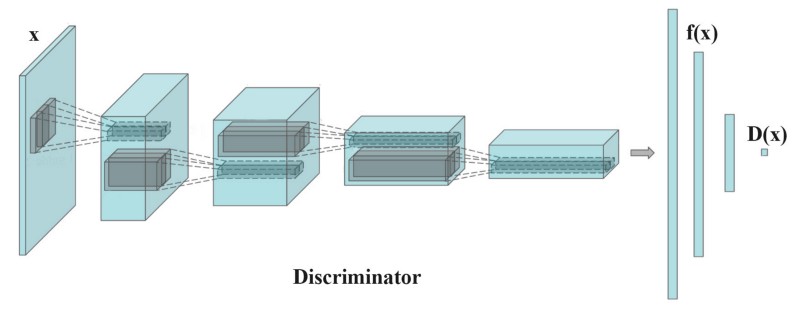
Feature-Matching

Feature-matching mediates “Non-convergence” and “Mode collapse” problems.

Feature matching changes the cost function for the generator to minimizing the statistical difference between the features of the real images and the generated images, using the L2-distance between the means of their feature vectors. It changes the goal from beating the opponent discriminator to matching the features of the real images. The new cost function for the generator is

$\| \mathbb{E}_{x \sim p_{\text{data}}} \mathbf{f}(\mathbf{x}) - \mathbb{E}_{z \sim p_z} \mathbf{f}(G(\mathbf{z})) \|^2_{L2}$

where $\mathbf{f}(x)$ is the feature vector extracted in an intermediate layer by the discriminator.

See https://github.com/raghav64/SemiSuper_GAN/blob/master/SSGAN.ipynb

# Discriminator
def discriminator():
    ...
    # Feature matched layer
    conv4 = tf.layers.conv2d(dropout3, 1024, kernel_size=[3,3], strides=[1,1],
                             padding='valid',activation = tf.nn.leaky_relu, name='conv4') # ?*2*

    # Applying Global average pooling
    features = tf.reduce_mean(conv4, axis = [1,2])

    ...

def build_GAN(x_real, z, dropout_rate, is_training):

    fake_images = generator(z, dropout_rate, is_training)

    D_real_features, D_real_logits, D_real_prob = discriminator(x_real, dropout_rate,
                                                              is_training)

    D_fake_features, D_fake_logits, D_fake_prob = discriminator(fake_images, dropout_rate,
                                                                is_training, reuse = True)
    #Setting reuse=True this time for using variables trained in real batch training

    return D_real_features, D_real_logits, D_real_prob, \
           D_fake_features, D_fake_logits, D_fake_prob, fake_images

def train():
    # G_L_1 -> Fake data wanna be real
    G_L_1 = tf.reduce_mean(tf.nn.sigmoid_cross_entropy_with_logits(
            logits = D_fake_logit[:, 0],
            labels = tf.zeros_like(D_fake_logit[:, 0], dtype=tf.float32)))

    # G_L_2 -> Feature matching
    data_moments = tf.reduce_mean(D_real_features, axis = 0)
    sample_moments = tf.reduce_mean(D_fake_features, axis = 0)
    G_L_2 = tf.reduce_mean(tf.square(data_moments-sample_moments))

    # Total loss
    G_L = G_L_1 + G_L_2

Minibatch Discrimination

Feeding real images and generated images separately into the discriminator in different batches and compute the similarity of the image $x$ with images in the same batch. We append the similarity $o(x)$ in one of the dense layers in the discriminator to classify whether this image is real or generated.

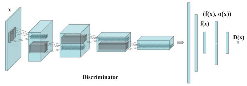
If mode starts to collapse, then similarity of $o(x_{\text{fake}})$ would increase. The discriminator can then penalize the generator if mode is collapsing.

The similarity between image $x_i$ and $x_j$ is computed as following

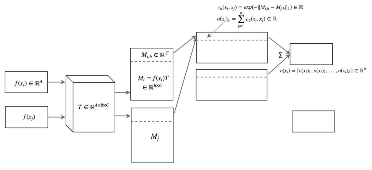
Given feature extraction layer of the discriminator $f(x_i) \in \mathbb{R}^A$, and transformation $T \in \mathbb{R}^{A \times B \times C}$

$M_i = f(x_i)T, M_j = f(x_j)T \in \mathbb{R}^{B \times C}$

$M_{i,b}, M_{j,b} \in \mathbb{R}^C$

$c_b(x_i, x_j) = \exp(-| M_{i,b} - M_{j,b}|_{L1}) \in \mathbb{R}$

$o(x_i)_b = \sum_\limits{j=1}^n c_b(x_i, x_j) \in \mathbb{R}$

$ o(x_i) = [o(x_i)_1, o(x_i)_2, …, o(x_i)_B] \in \mathbb{R}^B $

As a quote from the paper “Improved Techniques for Training GANs”

Minibatch discrimination allows us to generate visually appealing samples very quickly, and in this regard it is superior to feature matching.

One-sided label smoothing

Replacing $0$ and $1$ classifier targets with smoothe values like $0.1$ and $0.9$ seems to be effective to reduce vulnerability of neural networks to adversarial examples (this means, the GAN model may be overconfident and uses only a few features to predict the results).

Suppose we replace positive targets with $\alpha$ and negative with $\beta$, the optimal discriminator becomes

$D(x) = \frac{\alpha p_{\text{data}}(x) + \beta p_{\text{model}}(x)}{p_{\text{data}}(x) + p_{\text{model}}(x)}$

Only positive targets are replaced (hence one-sided). The negative targets remained $0$. This is because the presence of $p_{\text{model}}$ can be problematic, when $p_{\text{model}}$ is very large and $p_{\text{data}}$ is very small.

p = tf.placeholder(tf.float32, shape=[None, 10])
# Use 0.9 instead of 1.0.
feed_dict = {
  p: [[0, 0, 0, 0.9, 0, 0, 0, 0, 0, 0]] # Image with label "3"
}
# logits_real_image is the logits calculated by
# the discriminator for real images.
d_real_loss = tf.nn.sigmoid_cross_entropy_with_logits(
                    labels=p, logits=logits_real_image)

Historical Averaging

Keep track of model parameters for the last $T$ models (i.e. $\theta_{i-1}, \theta_{i-2}, …, \theta_{i-T}$). Then we use the historical model parameters to add an $L2$ regularisation term

$\|\theta_i - \frac{1}{T} \sum \limits_{t=1}^T \theta_{i-t} \|_{L2}$

For GANs with non-convex object function, historical averaging may stop models circle around the equilibrium point and act as a damping force to converge the model.

Virtual Batch Normaliztation (VBN)

Each example $x$ is normalized based on teh statistics collected on a reference batch of examples that are chosen once and fixed at the start of the training, and on $x$ itself, i.e.

$x_i = G(z_i, z_1, z_2, ..., z_n) \text{ instead of } x_i = G(z_i)$

where $z_i$ is the current batch, and $z_1$, $z_2$, … are the reference, pre-determined mini-batch. This combination will help prevent over-fitting (which will likely occur since we are reusing the reference batch over and over again).

VBN is computationally expensive since it requires running forward propagation on two minibatches of data. Only use in the generator network.

Change Cost Functions

The following figure lists the cost functions for some common GAN models.

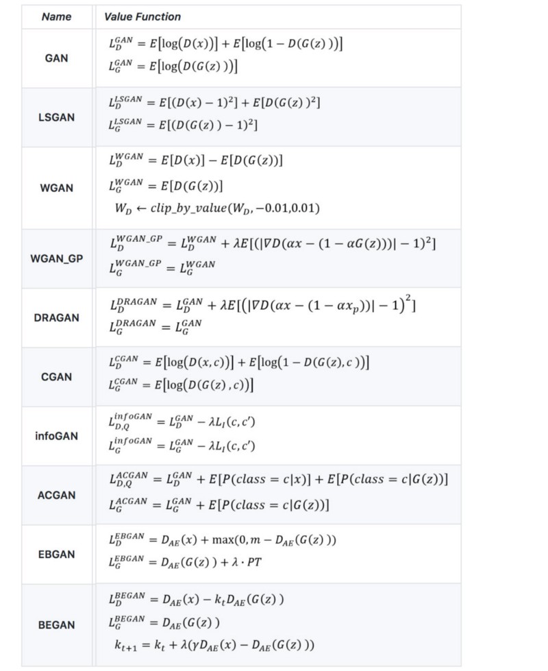
This is the last thing to consider. This link provides a comprehensive comparison of results using different cost functions.

Deep Video Portraits

The GAN version of DeepFake that can portrait sequences of videos: https://arxiv.org/pdf/1805.11714.pdf.

The architecture of DVP is the following

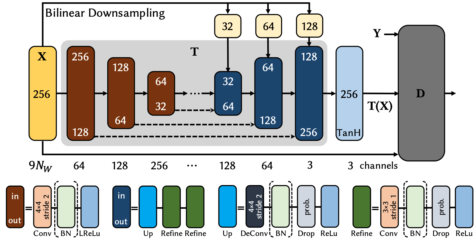
The area under the grey background is the auto-encoder $T$ for generating video sequences. It takes a $W \times H \times 9N_w$ space-time tensor $X$, where

$W$ is the width,
$H$ is the height
$9$ since there are 3 feature images, each has 3 color channels, total 9 images for each video frame
$N_w$ is the number of video frames (time component of the tensor). Used $N_w=11$ for this paper, hence they used 11 continuous frames (witht the current frame being the last of the stack) to ensure higher temporal coherence.

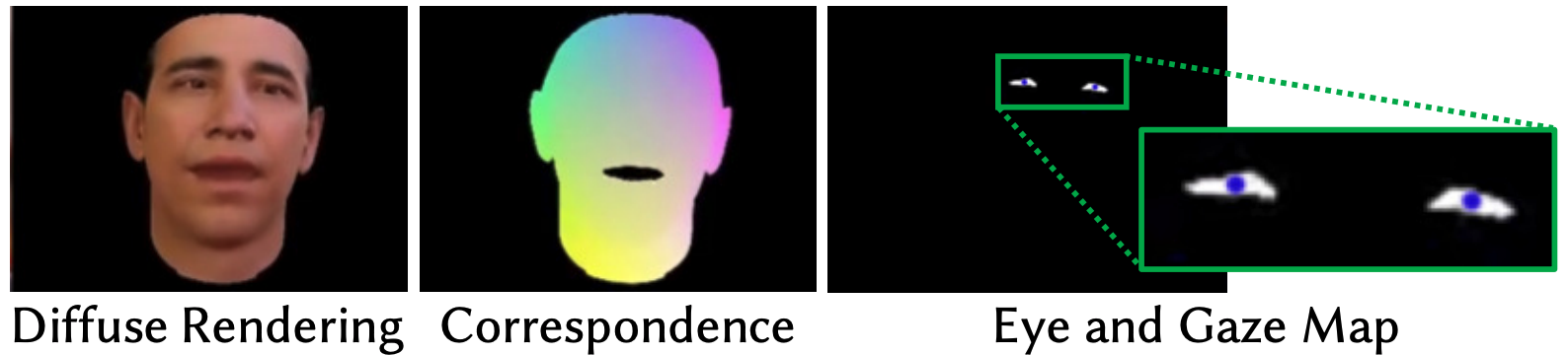
The 3 feature images are:

colored face rendering under target illumination
correspondence image encoding the index of the parametric face model’s vertex that projects into each pixel
eye gaze image that solely contains the white region of both eyes and the locations of pupils as blue circles

The output of the auto-encoder $T$ uses $\tanh$ activation to normalize the output between $-1$ and $1$ (i.e. black is $[-1, -1, -1]^T$, and white is $[+1, +1, +1]^T$). Recall the best-practice recommendations of GAN.

The objective function for the discriminator is

$T^* = \DeclareMathOperator*{\argmin}{argmin}\argmin \limits_T \max \limits_{D} E_{cGAN}(T, D) + \lambda E_{\ell_1}(T)$

where $E_{cGAN}$ is the adversarial loss

$E_{cGAN}(T,D) = \mathbb{E}_{X, Y} [\log D(X, Y)] + \mathbb{E}_X [\log (1-D(X, T(X)))]$

and $E_{\ell_1}(T)$ is an $\ell_1$ regularisation term that penalizes the distance between the synthesized image $T(X)$ and the ground-truth image $Y$,

$E_{\ell_1} = \mathbb{E}_{X,Y}[\|Y-T(X)\|_{L1}]$

PREVIOUSClassification of Seizure EEG with Convolutional Neural Network

NEXTDeep Learning Image Segmentation