We briefly review several types of problems that Expectation-Maximization algorithm was used to solve, including Mixture of Gaussian, Factor Analysis, and Latent Dirichlet Allocation.
Coin Flip Example
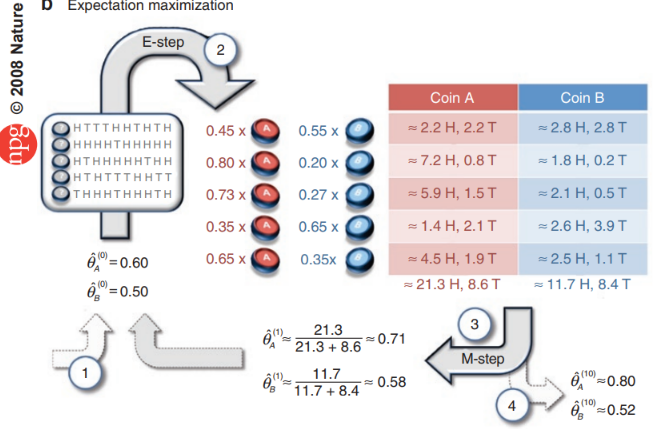
Suppose we have coin A and B. We first take a guess that the probability of of getting head for A is $\theta_A=0.6$, and probability of getting heads for B in $\theta_B=0.5$. This means, if we flip coin A and B 10 times each, we would expect 6 heads from A and 5 heads from B. In practice, we can guess or initialize $\theta_A$ and $\theta_B$ randomly.
Suppose we randomly pick a coin from the set of two coins for 10 times (with replacement) and flip the coin we picked, we get our first sample $x_1=[H, T, T, T, H, H, T, H, T, H]$. The hidden variable is $z \in {A, B}$ since we don’t know which coin we picked each time. The expectation maximization algorithm would help us estimate what $\theta$ and $z$ are using the observation $x$.
Expectation
The probability of getting 5 heads out of 10 coin flips, given a single flip has the probability of getting head is $\theta_A=0.6$, is:
$p(x_1 \mid z=A; \theta_A) = {10 \choose 5} (0.6)^5 (1-0.6)^5 = 0.200065 $
Similarly, for coin B ($\theta_B=0.5$), this is:
$p(x_1 \mid z=B; \theta_B) = {10 \choose 5} (0.5)^5 (1-0.5)^5 = 0.24609375$
We want to normalize the probability so that the total probability
$p(x_1 \mid z=A; \theta_A) + p(x_1 \mid z=B; \theta_B)=1$
This yields:
$p(x_1 \mid z=A; \theta_A) = \frac{0.2000065}{0.20065+0.24609375} = 0.45$
$p(x_1 \mid z=B; \theta_B) = 1-0.45=0.55$
This means, we estimated that A was taken 45% of the time (or 4.5 times), so that for the 5 heads observed, coin A contributed $0.45 \times 5 = 2.25$ heads on average.
Similarly, coin B was taken 55% of the time (or 5.5 times), so that for the 5 heads observed, coin B contributed $0.55 \times 5 = 2.75$ heads on average.
The “on average” term can be expressed by the expected value of the number of heads and tails for each coin, as the following:
$E[x_1=H \mid z=A] = x_1 p(x_1 \mid z=A; \theta_A) = 5\times 0.45=2.25$
$E[x_1=H \mid z=B] = x_1 p(x_1 \mid z=B; \theta_A) = 5\times 0.55=2.75$
$E[x_1=T \mid z=A] = x_1 p(x_1 \mid z=A; \theta_A) = 5\times 0.45=2.25$
$E[x_1=T \mid z=B] = x_1 p(x_1 \mid z=B; \theta_A) = 5\times 0.55=2.75$
Similarly, for $x_2 = [H, H, H, H, T, H, H, H, H, H]$, we do the same calculations
$p(x_2 \mid z=A; \theta_A) = {10 \choose 9}(0.6)^9(1-0.6)^1$
$p(x_2 \mid z=B; \theta_B) = {10 \choose 9}(0.5)^9(1-0.5)^1$
Normalize, we have
$p(x_2 \mid z=A; \theta_A) = 0.80$
$p(x_2 \mid z=B; \theta_B) = 1-0.80=0.20$
The expectations are:
$E[x_2=H \mid z=A] = x_2 p(x_2 \mid z=A; \theta_A) = 9\times 0.8=7.2$
$E[x_2=H \mid z=B] = x_2 p(x_2 \mid z=B; \theta_A) = 9\times 0.2=1.8$
$E[x_2=T \mid z=A] = x_2 p(x_2 \mid z=A; \theta_A) = 1\times 0.8=0.8$
$E[x_2=T \mid z=B] = x_2 p(x_2 \mid z=B; \theta_A) = 1\times 0.2=0.2$
Suppose we total have the following 5 samples / observations ${x_1, x_2, …, x_5}$. We find out the expected number of heads and tails for all 5 samples.
Maximization
We recalculate $\theta$, given the expected number of heads and tails from the above calculation. This is simply the total number of heads divided by the total number of coin flips (head + tail) for each coin.
$\theta_A = \frac{\sum_i x_ip(x_i=H \mid z=A)}{\sum_i x_ip(x_i=H \mid z=A) + \sum_i x_ip(x_i=T \mid z=A)} = \frac{21.3}{21.3+8.6} = 0.71$
$\theta_B = \frac{\sum_i x_ip(x_i=H \mid z=B)}{\sum_i x_ip(x_i=H \mid z=B) + \sum_i x_ip(x_i=T \mid z=B)} = \frac{11.7}{11.7+8.4} = 0.58$
In later formulations of EM algorithm, we shall see that this is actually maximizing the likelihood of $\theta$, i.e. $\DeclareMathOperator*{\argmax}{argmax} \argmax \limits_{\theta} L(\theta \mid x)$, where,
$L(\theta) = p(x; \theta) = \sum_z p(x, z; \theta) = \sum_z p(x \mid z; \theta)p(z;\theta)$
After obtaining the newly estimated $\theta$, we go back to the Expectation step and recalculate the expected number of heads and tails, which will then help us to estimate $\theta$. We repeat these two steps until $\theta$ converges to some value.
Mixture of Gaussian
To use EM algorithm to solve the Gaussian Mixture Model (GMM) problem, instead of picking and flipping coins, we are picking from Gaussian distributions and draw numbers from them.
Therefore, our hidden variable $z \in {\mathcal{N_1(\mu_1, s_1)}, \mathcal{N_2 (\mu_2, s_2)}, …}$, where $\mathcal{N_j}$ is the a Gaussian function parameterized by the mean $\mu_j$ and standard deviation $s_j$.
The data we are trying to model using Mixture of Gaussian can be seen to be generated in the following ways: for 1 data point, we randomly select a Gaussian function, and from that Gaussian function, we randomly select a number to make up the data point.
Therefore, the probability density of each data point $x_i$ generated by the $j$-th Gaussian function is normally distributed, i.e. $p(x_i \mid z_i=j) \sim \mathcal{N}_j(\mu_j, s_j)$ (for simplicity, from here on, let’s use $j$ to denote the $j$-th Gaussian $N_j$).
The GMM problem uses EM algorithm to estimate the parameters of each $\mathcal{N}_j(\mu_j, s_j)$, and the probability distribution of selecting each Gaussian function, i.e. $p(z) = \phi$. To estimate these parameters, we want to maximize their likelihood given the data $\mathbf{X}$.
To simplify our problem, let’s suppose we only have 2 Gaussians. In practice, the number of Gaussians need to be specified. $\phi = {\phi_1, \phi_2}$ where $\phi_1$ is the probability of selecting the 1st Gaussian function and $\phi_2$ is the probability of selecting the 2nd Gaussian. $\phi_1 + \phi_2 = 1$.
Let’s also define $\theta = {\phi, \mu, s}$.
The log-likelihood of $\theta$ is
To simplify, since $\phi$ does not parameterize $p(x_i \mid z)$, we change $p(x_i \mid z; \theta)$ to $p(x_i \mid z; \mu, s)$. $\mu$ and $s$ does not parameterize $p(z)$, we change $p(z;\theta)$ to $p(z; \phi)$. We then have
Maximum likelihood
To solve for this MLE problem, we initialize with the following assumption. Suppose all the data points are drawn from the 1st Gaussian function $\mathcal{N}_1(\mu_1, s_1)$,i.e. $z=1$. Then our log-likehood become
Optimizing $\ell$ by taking the derivative with respect to each and set the derivative to 0, we can obtain the follwoing:
$\phi_1 = \frac{1}{m}\sum_i^m I{z=1}$
$\mu_1 = \frac{\sum_i^m I{z=1}x_i}{\sum_i^m I{z=1}}$
$s_1 = \frac{\sum_i^m I{z=1}(x_i-u_1)(x_i-u_1)^T}{\sum_i^m I{z=1}}$
Operator $I$ is the indicator operator that indicates if $z==1$. For example, if $z=[1,2,1,1,2,1]$ (i.e., the first data point is drawn from the 1st Gaussian; the second data point is drawn from the 2nd Gaussian, etc..Then, $I{z=1}=[1,0,1,1,0,1]$, and $\sum_i^mI{z=1}=4$. Total number of data points $m=6$.
See the section at the end for the detailed derivation of these three solutions.
Expectation (E-Step)
We were able to simplify the MLE problem as above only because we made the assumption that all the data points are drawn from the 1st Gaussian. In reality, we want to calculate the probability that the data is from the 1st Gaussian, which we denote as $w$, and
Using Bayes’ Rule, $p(A \mid B) = \frac{p(B \mid A)p(A)}{p(B)}$, we can then calculate $w^{(i)}_1$ as
To calculate $p(x_i \mid z=1, \mu,s)$, we simply select the 1st Gaussian function, and then plugin the corresponding $x_i$.
$p(z=1 \mid \phi)$ is simply the probability of selecting the 1st Gaussian, i.e. $\phi_1$.
For the first iteration, we can take a random guess of the probability as well as the mean $\mu$ and standard deviation $s$. This is saying, the three parameters can be initialized with random numbers. It does not matter what the initial guesses are (as long as it is within the scale of these parameters, e.g. $\phi$ should be less than 1) since the algorithm can then update from the initial guesses to estimate the values more accurately anyway.
Maximization (M-step)
Replacing $I{z=1}$ with $w_1^{(i)}$, we have
$\phi_1 = \frac{1}{m}\sum_i^m w_1^i$
$\mu_1 = \frac{\sum_i^m w_1^i x_i}{\sum_i^m w_1^i}$
$s_1 = \frac{\sum_i^m w_1^i (x_i-u_1)(x_i-u_1)^T}{\sum_i^m w_1^i}$
We obtained 3 new estimations of the parameters. We then plug the newly estimated parameter back to the E-step. We repeat these two steps back and forth until the values of the parameters converge.
Simplifying the MLE problem
We want to maximize $\ell$ with respect to $\mu$, $s$, and $\phi$, separately
$\phi$:
We know that $p(z;\phi)$ is binomially distributed if there are only 2 Gaussian functions to select from. More generally, if we have $N$ Gaussian functions with $m$ observations, $p(z; \phi)$ is multinomially distributed. We also define $\sum_i^m I{z=j} = n_j$. Then,
$L(p(z;\phi)) = PDF(p(z;\phi)) = m! \cdot \prod_j \frac{p(z=j;\phi)^{n_j}}{n_j!}$
We also know that the total probability must be equal to 1, i.e. $C(p) = \sum_j p(z=j;\phi)=1$. This is a constraint for $L$. We then have the following Larange problem
$L(p) + \lambda C(p) = 0$
Taking the derivative on both sides, we have
More specifically,
Together, we have, $\frac{n_1}{p(z=1;\phi)} \cdot L = \lambda$, or $\frac{n_1}{p(z=1;\phi)} = \frac{\lambda}{L} = k$
Then, $n_1 = k \cdot p(z=1;\phi)$,
Similarly,$n_2 = k \cdot p(z=2;\phi)$,
Then, $\sum_j n_j = k \cdot \sum_j p(z=j; \phi)$
$m = k \cdot 1$,
$k = m$
Therefore, $\frac{\sum_i^m I{z=1}}{p(z=1;\phi)} = m$.
This means when $p(z=1;\phi) = \frac{\sum_i^m I{z=1}}{m}$,$L$ is maximized.
$\mu$ and $s$:
We know that $p(x_i\mid \mu, s) \sim \mathcal{N(\mu, s)}$. Let’s expand to $d$-dimensional multidimensional Gaussian function
where, $\Sigma = E[(x-\mu)(x-\mu)^T]$ is the covariance matrix. Then the likelihood function becomes
Then the log-likelihood become
Drop the $\frac{1}{2}$, we have
Taking the derivative relative to $\mu$, we have
This means,
$\sum_i^m (x_i-\mu) = \sum_i^m x_i - \sum_i^m \mu = \sum_i^m x_i - m\mu = 0$
$\mu = \frac{\sum_i^m x_i}{m}$
For the 2 Gaussian function,$\mu = {\mu_1, \mu_2}$, then,
$\frac{\partial}{\partial \mu_1} l \propto \sum_i^m (x_i - \mu \mid z=1) = 0$
$\sum_i^m (x_i \mid z=1) = \sum_i^m (\mu \mid z=1)$
$\sum_i^m I{z=1} x_i = \sum_i^m I{z=1} \mu_1$
$\mu_1 = \frac{\sum_i^m I{z=1}x_i}{\sum_i^m I{z=1}}$
$\frac{\partial}{\partial \Sigma} l = -\frac{\partial}{\partial \Sigma} \log(|\Sigma|) - \frac{\partial}{\partial \Sigma} \sum_i^m(x_i -\mu)^T \Sigma^{-1} (x_i - \mu) = 0$
With the following two known relationships,
$\frac{\partial}{\partial \Sigma}\log(|\Sigma|) = \Sigma^{-1} $
$\frac{\partial}{\partial \Sigma} (\sum_i^m (x_i-\mu)^T\Sigma^{-1}(x_i-\mu)) = -\sum_i^m \Sigma^{-1}(x_i-\mu)(x_i-\mu)^T\Sigma^{-1}$
Adding together, we have,
$\Sigma^{-1} = \sum_i^m \Sigma^{-1}(x_i-\mu)(x_i-\mu)^T\Sigma^{-1}$
$\Sigma = \sum_i^m(x_i-\mu)(x_i-\mu)^T$
Similar to $\mu_1$,
$\Sigma_1 = \frac{\sum_i^m I{z=1}(x_i-u)(x_i-\mu)^T}{\sum_i^m I{z=1}}$
# Generate some data
from sklearn.datasets.samples_generator import make_blobs
from sklearn.cluster import KMeans
import matplotlib.pyplot as plt
import numpy as np
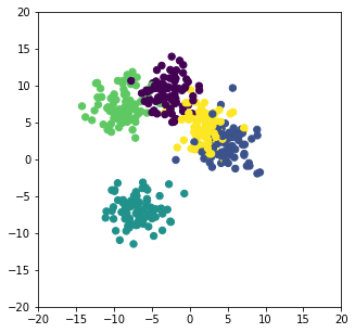
X, y_true = make_blobs(n_samples=400, centers=5, cluster_std=2., random_state=42)
plt.figure(figsize=(5,5))
plt.scatter(X[:,0], X[:, 1], c=y_true, s=40, cmap="viridis")
plt.xlim([-20,20])
plt.ylim([-20,20])
plt.show()
from matplotlib.patches import Ellipse
def draw_ellipse(position, covariance, ax=None, **kwargs):
    """Draw an ellipse with a given position and covariance"""
    ax = ax or plt.gca()

    # Convert covariance to principal axes
    if covariance.shape == (2, 2):
        U, s, Vt = np.linalg.svd(covariance)
        angle = np.degrees(np.arctan2(U[1, 0], U[0, 0]))
        width, height = 2 * np.sqrt(s)
    else:
        angle = 0
        width, height = 2 * np.sqrt(covariance)

    # Draw the Ellipse
    for nsig in range(1, 4): # draw 4 standard deviations
        ax.add_patch(Ellipse(position, nsig * width, nsig * height, angle, **kwargs))

def plot_gmm(gmm, X, label=True, ax=None):
    ax = ax or plt.gca()
    labels = gmm.fit(X).predict(X)
    if label:
        ax.scatter(X[:, 0], X[:, 1], c=labels, s=40, cmap='viridis', zorder=2)
    else:
        ax.scatter(X[:, 0], X[:, 1], s=40, zorder=2)
    ax.axis('equal')

    w_factor = 0.2 / gmm.weights_.max()
    for pos, covar, w in zip(gmm.means_, gmm.covariances_, gmm.weights_):
        draw_ellipse(pos, covar, alpha=w * w_factor)
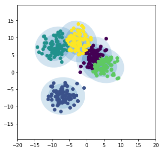
from sklearn.mixture import GaussianMixture
gmm = GaussianMixture(n_components=5)

plt.figure(figsize=(5,5))
plot_gmm(gmm, X)
plt.xlim([-20,20])
plt.ylim([-20,20])
plt.show()
General Formulation of EM algorithm
Jensen’s inequality
For concave function $f(x)$, with concave meaning the second derivative $f’‘(x) \le 0$ or Hessian $H \le 0$, we have the Jensen’s inequality
With the equality true if and only if $X = E[X]$and $\sum_x p(x)=1$, i.e. $X$ is constant.
EM algorithm
The type of problem that EM algorithm can solve can be generally formulated as the maximum likelihood problem with a latent variable $z$, such that
Now, suppose the $Q_i$ be some distribution over $z$, where $\sum_z Q_i(z) = 1$, and $Q_i (z) \ge 1$, then
For the equality condition to be true, we must choose $X$ to be constant, which means
$X = \frac{p(x^{(i)}, z^{(i)}; \theta)}{Q_i(z^{(i)})} = c$, or $Q_i(z^{(i)}) \propto p(x^{(i)}, z^{(i)}; \theta)$. Since $\sum_z Q_i(z^{(i)}) = 1$, we must have
Therfore, the EM algorithm can be carried out with the following 2 steps
Repeat until convergence {
(E-step) For each $i$, set
$Q_i(z^{(i)}) := p(z^{(i)} \mid x^{(i)}; \theta)$
(M-step) Set
$\DeclareMathOperator*{\argmax}{argmax} \theta := \argmax \limits_{\theta} \sum_i \sum_{z^{(i)}} Q_i (z^{(i)}) \log \frac{p(x^{(i)}, z^{(i)}; \theta)}{Q_i(z^{(i)})}$
}
In a GMM model, we would select $Q_i = w_i$.
Variational EM
From http://willwolf.io/2018/11/11/em-for-lda/, and C. M. Bishop. Pattern recognition and machine learning.
Recall the general formulation of EM
$Q_i(z^{(i)})$ is called variational distribution. It can be seen that,
$\sum_i \log p(x^{(i)}; \theta) = \sum_i \mathrm{E}_{z^{(i)} \sim Q_i} \Bigg[\log\Big(\frac{p(x^{(i)}, z^{(i)}; \theta)}{Q_i(z^{(i)})}\Big) \Bigg] + R$
Therefore,
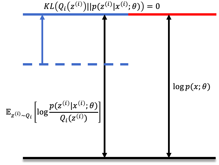
$\sum_i \log p(x^{(i)}; \theta) = \sum_i \mathrm{E}_{z^{(i)} \sim Q_i} \Bigg[\log\Big(\frac{p(x^{(i)}, z^{(i)}; \theta)}{Q_i(z^{(i)})}\Big) \Bigg] + \sum_i KL(Q_i(z^{(i)}) | p(z^{(i)} \mid x^{(i)}; \theta))$
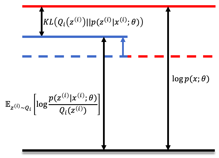
Graphicaly, this is represented as the following:
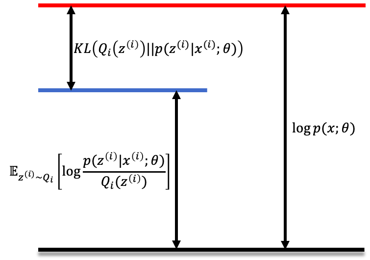
At the E-step, we fix $\theta$, and set $Q_i(z^{(i)}):=p(z^{(i)} \mid x^{(i)};\theta)$, such that $KL(Q_i(z^{(i)}) | p(z^{(i)} \mid x^{(i)};\theta) \rightarrow 0$. Therefore, this is equivalent to minimzing the $KL$ divergence with respect to $z^{(i)}$. As illustrated below, the blue arrow indicates the update of the lower bound at the E-step.
At the M-step, we hold the newly set $Q_i(z^{(i)})$ as a constant. We adjuste $\theta$ to maximize lower bound of the log-likelihood, illustrated below. The blue arrow indicates the update of the lower bound at M-step
Hidden Markov Model
The Hidden Harkov Model (HMM) tries to solve the following problem:
Suppose we have a set of observations over time ${x_1, x_2, …, x_t }$ generated by a distribution $V$. The distribution $V$ also depends on a state $z$ which are generated by a distribution $S$.
Let’s define $P(x_t = v_k \mid z_t = s_j) = B_{jk}$, i.e. when we are in state $z_t = s_j$, the probability of the observation $x_t = v_k$ is denoted by the matrix $B$. $B_{jk}$ is called the emission probability.
Let’s also define the state transition $P(z_t = s_j \mid z_{t-1}= s_i) = A_{ij}$, i.e. the probability of transition from state $s_i$ at time $t-1$ into $s_j$ at time $t$ is given by the matrix $A$. $A_{ij}$ is called the transition probability.
Since we are under Markov asummption, the current value and state only depends on the value and state of the previous state, meaning $p(\mathbf{x}) = p(x_t, x_{t-1}, …, x_1) = p(x_t \mid x_{t-1})p(x_{t-1} \mid x_{t-2})…p(x_2 \mid x_1)$.
The HMM problem tries to esitmate $A$ and $B$ given the data $\mathbf{x}$. Essentially, this is maximizing the likelihood
With constraints
where $|V|, |S|$ denotes the number of values that distributions $V, S$ can take, respectively.
We then have the Lagrange problem
For details on how to apply EM to estimate this likelihood, see Section notes on HMM from Andrew Ng’s Machine Learning course.
# Example using hmmlearn, which is separated out from sklearn
import numpy as np
import datetime
from matplotlib import cm, pyplot as plt
from matplotlib.dates import YearLocator, MonthLocator, date2num

import pandas_datareader.data as web
import pandas_datareader
from hmmlearn.hmm import GaussianHMM

import warnings # try to suppress some warnings
from IPython.display import display

np.random.seed(42)

# Get data from Ford
f = web.DataReader("F", "morningstar", datetime.datetime(2010, 1,1), datetime.datetime(2013,1,27))
display(f.head())
display(f.tail())

# Take diff of close value. Note that this makes
# ``len(diff) = len(close_t) - 1``, therefore, other quantities also
# need to be shifted by 1.
diff = np.diff([float(v) for v in f['Close'].values])
volume = f['Volume'].values[1:]
dates = np.asarray([date2num(i[1].date()) for i in f.index])[1:]
close_v = f['Close'][1:]
X = np.column_stack([diff, volume])
| Close | High | Low | Open | Volume | ||
|---|---|---|---|---|---|---|
| Symbol | Date | |||||
| F | 2010-01-01 | 10.00 | 10.06 | 9.9200 | 10.04 | 0 |
| 2010-01-04 | 10.28 | 10.28 | 10.0455 | 10.17 | 60855796 | |
| 2010-01-05 | 10.96 | 11.24 | 10.4000 | 10.45 | 215620138 | |
| 2010-01-06 | 11.37 | 11.46 | 11.1300 | 11.21 | 200070554 | |
| 2010-01-07 | 11.66 | 11.69 | 11.3200 | 11.46 | 130201626 |
| Close | High | Low | Open | Volume | ||
|---|---|---|---|---|---|---|
| Symbol | Date | |||||
| F | 2013-01-21 | 14.11 | 14.11 | 14.11 | 14.11 | 0 |
| 2013-01-22 | 14.17 | 14.19 | 14.00 | 14.06 | 35475103 | |
| 2013-01-23 | 13.88 | 14.02 | 13.79 | 14.00 | 58122134 | |
| 2013-01-24 | 13.87 | 13.98 | 13.81 | 13.82 | 42536100 | |
| 2013-01-25 | 13.68 | 13.84 | 13.64 | 13.83 | 53405308 |
# Make an HMM instance and execute fit
model = GaussianHMM(n_components=4, covariance_type="diag", n_iter=1000) # 4 hidden states
warnings.filterwarnings("ignore", category=DeprecationWarning)
model.fit(X)
# Predict the optimal sequence of internal hidden state
hidden_states = model.predict(X)
print("hidden states:\n" , hidden_states)
print("transition matrix:\n", model.transmat_)

print("Means and vars of each hidden state")
for i in range(model.n_components):
    print("{0}th hidden state".format(i))
    print("mean = ", model.means_[i])
    print("var = ", np.diag(model.covars_[i]))
    print()
hidden states:
 [1 3 3 3 3 3 3 3 3 3 3 1 1 3 3 3 3 3 3 3 1 1 1 3 3 1 1 1 2 2 0 2 2 2 2 2 1
 1 1 1 3 3 3 1 1 1 1 2 2 1 1 1 3 3 3 3 3 1 1 1 3 3 3 3 3 1 1 1 1 2 2 1 3 3
 3 1 1 1 1 1 3 3 3 3 3 3 3 3 3 3 3 3 1 1 1 1 1 3 3 3 3 3 3 1 1 3 1 1 1 1 1
 1 1 2 2 2 2 2 2 2 2 1 1 1 3 3 3 3 3 3 3 1 1 2 2 2 1 2 2 2 2 2 2 1 3 3 1 2
 1 1 1 1 2 2 2 2 2 2 2 2 2 2 2 2 2 2 1 1 2 2 2 2 1 2 2 0 0 0 0 0 0 0 2 1 2
 2 2 2 2 2 0 0 0 0 2 1 1 1 2 2 2 2 2 2 2 2 1 1 1 2 1 3 1 2 2 2 2 3 3 3 3 3
 3 1 1 3 3 3 3 3 1 1 2 0 0 2 2 1 1 2 2 2 1 2 2 2 2 2 2 2 0 0 0 0 0 0 0 0 0
 0 1 1 1 1 1 2 2 1 1 2 0 0 1 1 2 2 2 1 1 3 3 3 3 3 1 1 2 2 2 1 2 2 2 2 2 0
 1 3 1 1 2 2 2 2 1 1 1 1 1 1 1 1 1 1 2 2 2 2 1 2 0 0 0 0 1 1 1 2 2 2 1 1 2
 2 2 2 2 2 2 0 2 3 1 2 2 2 2 2 2 2 0 0 2 2 2 2 2 2 2 2 2 2 1 2 0 0 2 1 2 2
 2 2 2 2 1 1 1 1 1 1 2 2 2 2 1 2 2 2 2 2 0 2 2 2 2 2 2 2 2 2 2 2 0 0 0 0 1
 1 1 1 1 1 3 3 3 3 3 3 1 1 2 2 2 1 1 1 2 2 2 2 2 2 2 2 2 0 2 2 2 2 2 2 2 2
 2 2 2 2 1 2 2 2 2 2 2 1 1 1 1 1 2 2 1 2 2 2 2 2 2 1 1 1 3 1 2 2 1 2 2 2 2
 2 1 2 0 0 0 2 2 2 2 2 2 0 0 2 2 2 2 2 2 2 2 1 2 2 2 2 2 2 2 2 2 2 0 0 0 0
 0 0 0 2 2 2 2 2 1 2 2 0 0 0 2 2 2 2 2 2 1 1 2 2 2 2 1 2 0 0 2 2 0 0 0 2 0
 0 0 0 0 0 0 0 2 2 2 2 2 0 0 0 0 2 2 2 1 2 0 0 0 0 0 0 0 0 0 2 1 2 0 0 2 2
 0 0 0 0 0 0 0 0 0 0 2 2 2 2 2 2 2 2 0 0 0 0 0 2 2 2 2 2 2 2 2 2 0 0 2 2 2
 2 2 2 2 0 0 0 0 0 0 0 0 0 0 2 2 2 0 0 0 1 2 2 0 0 0 0 0 0 0 0 0 0 0 0 0 0
 2 2 2 2 0 0 0 0 0 0 0 0 0 0 0 0 0 0 0 0 0 0 0 0 0 0 0 0 0 0 0 0 2 2 0 0 0
 2 2 0 0 0 0 0 0 0 0 0 0 0 2 2 2 0 0 0 0 0 0 0 0 0 0 0 0 0 2 2 0 0 0 1 1 2
 2 2 2 2 0 0 0 2 2 2 2 0 0 0 0 0 0 0 2 0 0 0 0 0 0 0 0 0 0 0 2 2 2 2 1 1 3
 3 1 1 1 3 1 1 2 2 2 2 1 2 2 2 2 0 0 0 0 2 2 2]
transition matrix:
 [[  7.62209081e-01   4.42763798e-02   1.93514540e-01   2.12193069e-36]
 [  6.86788107e-13   5.29018945e-01   3.34975742e-01   1.36005312e-01]
 [  1.72871887e-01   1.40790045e-01   6.76955667e-01   9.38240077e-03]
 [  9.17429797e-66   2.60686279e-01   1.83075401e-48   7.39313721e-01]]
Means and vars of each hidden state
0th hidden state
mean =  [ -9.50707573e-03   3.23468863e+07]
var =  [  1.20319939e-02   1.91006372e+14]

1th hidden state
mean =  [  3.07023385e-02   8.87799105e+07]
var =  [  1.08007116e-01   3.86670786e+14]

2th hidden state
mean =  [  1.32939629e-02   5.42620776e+07]
var =  [  4.01014371e-02   1.07809100e+14]

3th hidden state
mean =  [ -3.52229820e-02   1.49437693e+08]
var =  [  2.44416859e-01   5.56821850e+15]


D:\Anaconda3\lib\site-packages\hmmlearn\base.py:459: RuntimeWarning: divide by zero encountered in log
  np.log(self.startprob_),
D:\Anaconda3\lib\site-packages\hmmlearn\base.py:468: RuntimeWarning: divide by zero encountered in log
  np.log(self.startprob_),
D:\Anaconda3\lib\site-packages\hmmlearn\base.py:451: RuntimeWarning: divide by zero encountered in log
  n_samples, n_components, np.log(self.startprob_),
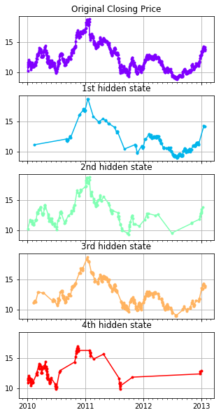
fig, axs = plt.subplots(model.n_components+1, sharex=True, sharey=True, figsize=(5,10))
num_states = ['1st', '2nd', '3rd', '4th']
colours = cm.rainbow(np.linspace(0, 1, model.n_components+1))

axs[0].plot_date(dates, close_v, ".-", c=colours[0])
axs[0].set_title("Original Closing Price")
for i, ax in enumerate(axs[1:]):
    # Use fancy indexing to plot data in each state.
    mask = hidden_states == i
    ax.plot_date(dates[mask], close_v[mask], ".-", c=colours[i+1])
    ax.set_title("{} hidden state".format(num_states[i]))

# Format the ticks.
for ax in axs:
    ax.xaxis.set_major_locator(YearLocator())
    ax.xaxis.set_minor_locator(MonthLocator())
    ax.grid(True)

plt.show()
Special Note
Check out PyMC3, a Python package for Bayesian statistical modeling and Probabilistic Machine Learning focusing on advanced Markov chain Monte Carlo (MCMC) and variational inference (VI) algorithms.
Factor Analysis
Factor analysis a dimensionality reduction technique. It is similar to PCA.
Marginal and Conditional Probabilities of Gaussian
Given the $\mathbf{x} = \begin{bmatrix} x_1 \ x_2\end{bmatrix}$
where $x_1 \in \mathbb{R}^r$, $x_2 \in \mathbb{R}^s$, and $x \in \mathbb{R}^{r+s}$.
Suppose $x \sim \mathcal{N}(\mathbf{\mu}, \mathbf{\Sigma})$, then $\mathbf{\mu} =\begin{bmatrix} \mu_1 \ \mu_2 \end{bmatrix}$ and $\mathbf{\Sigma} = \begin{bmatrix} \Sigma_{11} & \Sigma_{12} \ \Sigma_{21} & \Sigma_{22} \end{bmatrix}$, where $\mu_1 \in \mathbb{R}^r$, $\mu_2 \in \mathbb{R}^s$, $\Sigma_{11} \in \mathbb{R}^{r \times r}$, $\Sigma_{22} \in \mathbb{R}^{s \times s}$, and $\Sigma_{12}=\Sigma_{21}^T \in \mathbb{R}^{r \times s}$.
We can see that $E[x_1] = \mu_1$, and $Cov(x_1) = E[(x_1 - \mu_1)(x_1 - \mu_1)] = \Sigma_{11}$
This means, the marginal probabilities
For the conditional probability $p(x_1 \mid x_2) = \mathcal{N}(\mu_{1 \mid 2}, \Sigma_{1 \mid 2})$, where
Formulation of Factor Analysis
We posit a joint distribution on $(x, z)$, where $x \in \mathbb{R}^n$ and $z \in \mathbb{R}^k$ is a latent variable, with distributions
$\Psi$ is a diagnoal matrix. We want to calculate the marginal and conditional probability distributions, i.e. $p(x \mid z)$ and $p(x, z)$. We define the joint distribution as
From the above relationships, we know that $\mu_{zx} = \begin{bmatrix} \vec{0} \ \mu \end{bmatrix}$, $\Sigma_{zz} = I$, and
Similarly,
Therefore,
The marginal distribution of $p(x) = \mathcal{N}(\mu, \Lambda \Lambda^T + \Psi)$. We want to maximize the log-likelihood of $p(x)$, given the parameters $\mu, \Lambda, \Psi$, i.e.
EM Algorithm to solve the factor analysis problem
To maximize the log-likelihood iteratively using EM algorithm, we start with the general form of problem that can be solved with EM:
E-Step
We select $Q_i(z^{(i)}) = p(z^{(i)} \mid x; \mu, \Lambda, \Psi)$. From the conditional probability formula above, we have $p(z^{(i)} \mid x; \mu, \Lambda, \Psi) = \mathcal{N}(\mu_{z^{(i)} \mid x^{(i)}}, \Sigma_{z^{(i)} \mid x^{(i)}})$, where
Plugging in for $Q_i(z^{(i)})$
M-Step
We maximize the log-likelihood $\ell$ with respect to $\mu, \Lambda, \Psi$.
We can drop the terms $\log(p(z^{(i)})$ and $\log Q_i(z^{(i)})$ since they are not dependent on the parameters. Therefore, we only need to maximize
Again, from the above formula on conditional distribution
Plugging in, we have
$\mu$:
We will take derivative of the last term with respect to $\mu$. We will take advantage of the fact that $\frac{\partial}{\partial s}(x-s)^T W (x-s) = -2W(x-s)$ (Matrixcookbook 2.4.2 formula 86). Then,
$\frac{-\frac{1}{2}(x^{(i)}-\mu-\Lambda z^{(i)})^T \Psi^{-1} (x^{(i)}-\mu-\Lambda z^{(i)})}{\partial \mu} = -\frac{1}{2} \cdot -2 \Psi^{-1} \cdot (x^{(i)}-\mu-\Lambda z^{(i)})$
Solve, we have
$\sum_{i=1}^m E_{z^{(i)} \sim Q_i} \big[x^{(i)}- \mu - \Lambda z^{(i)} \big] = 0$
$\sum_{i=1}^m x^{(i)}- \mu - E_{z^{(i)} \sim Q_i} \big[\Lambda z^{(i)} \big] = 0$
since
$\sum_{i=1}^m x^{(i)} = \sum_{i=1}^m \mu = m \cdot \mu$
$\mu := \frac{1}{m} \sum_{i=1}^m x^{(i)}$
Notice the $\mu$ only need to be calculated once.
$\Lambda$:
We again only take the derivative of the last term, but with $\Lambda$ this time. We will take advantage of the fact that $\frac{\partial}{\partial A}(x-As)^T W (x-As) = -2 W(x-As)s^T$ (Matrixcookbook 2.4.2 formula 88). Then,
$\frac{-\frac{1}{2}(x^{(i)}-\mu-\Lambda z^{(i)})^T \Psi^{-1} (x^{(i)}-\mu-\Lambda z^{(i)})}{\partial \Lambda} = -\frac{1}{2} \cdot -2 \Psi^{-1} \cdot (x^{(i)}-\mu-\Lambda z^{(i)}) (z^{(i)})^T$
Then,
$\sum_{i=1}^m E_{z^{(i)} \sim Q_i} \big[(x^{(i)}-\mu)(z^{(i)})^T - \Lambda z^{(i)}(z^{(i)})^T \big] = 0$
$\sum_{i=1}^m (x^{(i)}-\mu) E_{z^{(i)} \sim Q_i} \big[(z^{(i)})^T\big] = \Lambda \sum_{i=1}^m E_{z^{(i)} \sim Q_i} \big[z^{(i)}(z^{(i)})^T\big] $
$\Big(\sum_{i=1}^m (x^{(i)}-\mu) \cdot E_{z^{(i)} \sim Q_i} \big[(z^{(i)})^T\big] \Big) \Big(\sum_{i=1}^m E_{z^{(i)} \sim Q_i} \big[z^{(i)}(z^{(i)})^T\big] \Big)^{-1} = \Lambda $
Since $z^{(i)}$ is sampled from $Q_i$, $E_{z^{(i)} \sim Q_i} \big[(z^{(i)})^T\big] = \mu^T_{z^{(i)} \mid x^{(i)}}$
For $E_{z^{(i)} \sim Q_i} \big[z^{(i)}(z^{(i)})^T\big]$, we take advantage of the fact $Cov(Y) = E[YY^T] - E[Y]E[Y]^T \rightarrow E[YY^T] = E[Y]E[Y]^T + Cov(Y)$, then
$E_{z^{(i)} \sim Q_i} \big[z^{(i)}(z^{(i)})^T\big] = \mu_{z^{(i)} \mid x^{(i)}} \cdot \mu^T_{z^{(i)} \mid x^{(i)}} + \Sigma^T_{z^{(i)} \mid x^{(i)}} $
Plugging everything back in, we have
$\Lambda := \Big(\sum_{i=1}^m (x^{(i)}-\mu) \cdot \mu^T_{z^{(i)} \mid x^{(i)}} \Big) \Big(\sum_{i=1}^m \mu_{z^{(i)} \mid x^{(i)}} \cdot \mu^T_{z^{(i)} \mid x^{(i)}} + \Sigma^T_{z^{(i)} \mid x^{(i)}} \Big)^{-1}$
$\Psi$:
We need to take the derivative with respect to the last two terms
For the second to last $\log$ term, we take advantage of the fact $\frac{\partial \log |X|}{\partial X} = X^{-T}$ (matrix cookbook Section 2.1.4 Equation 57)
For the last term, we take advantage of the fact $\frac{\partial a^TX^{-1}a}{\partial X} = -X^{-T}aa^TX^{-T}$ (matrix cookbook Section 2.3 Equation 61)
Together, we have
$-\frac{1}{2} \Psi^{-T} + \frac{1}{2}\Psi^{-T}(x^{(i)}-\mu-\Lambda z^{(i)})(x^{(i)}-\mu-\Lambda z^{(i)})^T \Psi^{-T} = 0$
$\Psi^{-T} = \Psi^{-T}(x^{(i)}-\mu-\Lambda z^{(i)})(x^{(i)}-\mu-\Lambda z^{(i)})^T \Psi^{-T}$
$\Psi^T \Psi^{-T} \Psi^T = \Psi^T \Psi^{-T}(x^{(i)}-\mu-\Lambda z^{(i)})(x^{(i)}-\mu-\Lambda z^{(i)})^T \Psi^{-T} \Psi^T$
$\Psi^T = (x^{(i)}-\mu-\Lambda z^{(i)})(x^{(i)}-\mu-\Lambda z^{(i)})^T$
$\Psi = (x^{(i)}-\mu-\Lambda z^{(i)})(x^{(i)}-\mu-\Lambda z^{(i)})^T$ (consider $(AB)^T = B^T A^T$)
Adding the summation term
$\sum_{i=1}^m E_{z^{(i)} \sim Q_i} [\Psi] = \sum_{i=1}^m E_{z^{(i)} \sim Q_i} \big[(x^{(i)}-\mu-\Lambda z^{(i)})(x^{(i)}-\mu-\Lambda z^{(i)})^T \big]$
For the last two terms,
The constant term can be dropped since it does not depende on $x^{(i)}$. Also, since $\Psi$ is a diagonal matrix, take the diagonal terms in the above calculation when updating $\Psi$.
# Example factor analysis: looking for hidden factors
from sklearn.datasets import load_iris
from sklearn.decomposition import FactorAnalysis

iris = load_iris()
X, y = iris.data, iris.target
factor = FactorAnalysis(n_components=4, random_state=101).fit(X) # looking at 4 factors
import pandas as pd
df = pd.DataFrame(factor.components_, columns=iris.feature_names)
df
# The max number of coponents should be 2, not 4
| sepal length (cm) | sepal width (cm) | petal length (cm) | petal width (cm) | |
|---|---|---|---|---|
| 0 | 0.707227 | -0.153147 | 1.653151 | 0.701569 |
| 1 | 0.114676 | 0.159763 | -0.045604 | -0.014052 |
| 2 | -0.000000 | 0.000000 | 0.000000 | 0.000000 |
| 3 | -0.000000 | 0.000000 | 0.000000 | -0.000000 |
Latent Dirichlet Allocation (LDA)
LDA is a generative model that tries to find topics of given a list of documents. In LDA, we assume the documents are generated in the following process:
- Each document has a distribution of topics.
- Each topic has a distribution of words.
- To generate a document
- Select a topic based on the distribution
- From that topic, select a word based on the distribution (unigram bag-of-words)
This, of course, disregards any order of words (hence, bag-of-words).
To determine the topics, we go backwards in this process. Since we observe the words that are generated, we want to infer the topic selected (in a probabilistic fashion). From the inferred topic selected, we can determine the distribution of topics.
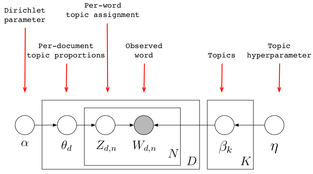
More formally, we have the following model (with plate notation)
Or expressed as a joint probability,
where
- $K$: Number of topics a document belongs to (a fixed number);
- $N$: Number of words in each document;
- $D$: Number of documents;
- $\vec{\theta}_d$: the topic proportions vector for document $d$;
- $\theta_{d, k}$: the topic proportion for topic $k$ in document $d$;
- $\vec{z}_d$: the topic assignments for document $d$. For example it might be, Animal = (0.3 Cats, 0.4 Dogs, 0 AI, 0.2 Loyal, 0.1 Evil);
- $z_{d,n}$: the topic assignment for word $n$ in document $d$; $z_{d,n}$ is multinomially distributed with proprotions specified by $\theta{d, k}$
- $\vec{w}_d$: the observed words for document $d$;
- $w_{d,n}$: the $n$-th observed word for document $d$. This is the only observation;
- $\vec{\beta}_k$: the distribution of vocabularies for topic $k$;
- $\beta_{k, v}$: the probability of vocabulary $v$ under topic $k$;
- $\alpha$: the parameter for the distribution of $\theta$. We assume it is Dirichlet;
- $\eta$: the parameter for the distribution of $\beta$. We assume it is Dirichlet.
Dirichlet distribution
Dirichlet distribution is the multi-dimensional generalization of Beta distribution. Just like Beta distribution is the conjugate prior of the Bernouli, Binomial, Negative Binomial, or Geometric distributions (all binary cases), Dirichlet distribution is the conjuate prior for Multinomial distribution (multiple cases).
Beta distribution is in fact, a special case of Dirichlet distribution, with only 2 parameters (just like binomial disitrubiton is a special case for multinomial distribution). Dirichlet distribution can have more than 2 parameters.
For both Dirichelt and Beta distribution, we can consider them as a distribution over distributions.
A quick review of conjugate prior, Binomial and Beta distribution
Recall Bayes’ theorem
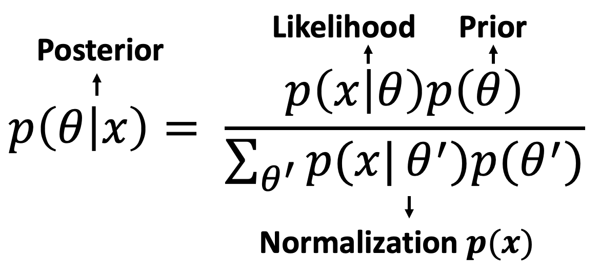
where $p(\theta)$ is calle the prior (the prior belief of $\theta$ before oberving $x$), $p(x \mid \theta)$ is called the likelihood, and $p(\theta \mid x)$ is called the posterior (after observing $x$). The sum in the bottom is a normalizing factor, or essentially $p(x)$.
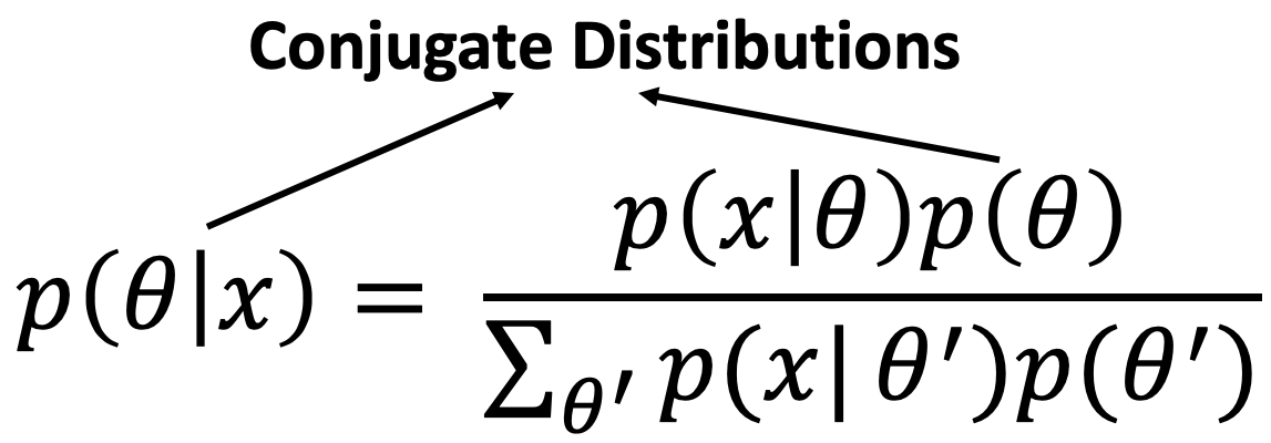
If the posterior $p(\theta \mid x)$ is in the same probability distribution family as the prior $p(\theta)$, then $p(\theta)$ is a special type of prior called conjugate prior (conjugate to the likelihood $p(x \mid \theta)$). $p(\theta \mid x)$ and $p(\theta)$ are a pair of conjugate distributions.
An analogy of this is eigen vectors: $A \nu = \lambda \nu$. The eigen vector $\nu$ to matrix $A$ is like the conjugate prior $p(\theta)$ to likelihood function $p(x \mid \theta)$.
In the case of binomial / beta distributions: if the likelihood $p(x \mid \theta) $ is binomial and prior $p(\theta)$ is beta distribution, then the posterior $p(\theta \mid x)$ is also beta distribution.
The following results are from https://ocw.mit.edu/courses/mathematics/18-05-introduction-to-probability-and-statistics-spring-2014/readings/MIT18_05S14_Reading15a.pdf
Binomial
| hypothesis | data | prior | likelihood | posterior |
|---|---|---|---|---|
| $\theta$ | $x$ | $\beta(a, b)$ | $binomial(N, \theta)$ | $\beta(a+x, b+N -x)$ |
| $\theta$ | $x$ | $c_1 \theta^{a-1}(1-\theta)^{b-1}$ | $c_2 \theta^x (1 − \theta)^{N−x}$ | $c_3 \theta^{a+x−1} (1 − \theta)^{b+N−x−1}$ |
where $c_1$, $c_2$, and $c_3$ are corresponding distribution normalizing factors: $c_1 = \frac{(a+b-1)!}{(a-1)!(b-1)!}$, $c_2={N \choose x} = \frac{N!}{(N-x)!x!}$, $c_3=\frac{(a+b+N-1)!}{(a+x-1)!(b+N-x-1)!}$
Bernouli
| hypothesis | data | prior | likelihood | posterior |
|---|---|---|---|---|
| $\theta$ | $x$ | $\beta(a, b)$ | Bernoulli($\theta$) | $\beta(a+1, b)$ or $\beta(a, b+1)$ |
| $\theta$ | $x=1$ | $c_1 \theta^{a-1}(1-\theta)^{b-1}$ | $\theta$ | $c_3 \theta^{a} (1-\theta)^{b-1}$ |
| $\theta$ | $x=0$ | $c_1 \theta^{a-1}(1-\theta)^{b-1}$ | $1-\theta$ | $c_3 \theta^{a-1} (1-\theta)^{b}$ |
For $c_1$ and $c_3$, set $N=1$ for the above binomial case.
Multinomial and Dirichlet distribution
| hypothesis | data | prior | likelihood | posterior |
|---|---|---|---|---|
| $\alpha, \theta$ | $x$ | $p(\theta) = Dir(\alpha)$ | $p(x \mid \theta) = multinomial(\theta)$ | $p(\theta \mid x) = Dir(\alpha + x)$ |
| $\alpha, \theta$ | $x$ | $c_1 \prod_{i=1}^d \theta_i^{\alpha_i -1}$ | $c_2 \prod_{i=1}^d \theta_i^{x_i}$ | $c_3 \prod_{i=1}^d \theta_i^{x_i + \alpha_i-1}$ |
where $c_1=\frac{\Gamma \sum_{i=1}^d \alpha_i}{\prod_{i=1}^d \Gamma(\alpha_i)}$, $c_2=\frac{(\sum_{i=1}^d x_i)!}{\prod_{i=1}^d x_i !} \prod_i^d \theta^{x_i} = \frac{\Gamma(\sum_{i=1}^d x_i+1)}{\prod_{i=1}^d \Gamma (x_i+1)}$, $c_3 \propto c_1 \cdot c_2$.
See https://mast.queensu.ca/~communications/Papers/msc-jiayu-lin.pdf for more mathematical details on Dirichlet distribution.
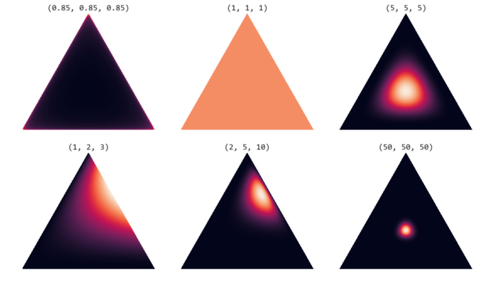
Here is an example of Dirichlet distribution with 3 parameters.
Maximizing the Posterior with Variational EM
From http://willwolf.io/2018/11/11/em-for-lda/
Recall the general formulation of EM
Our joint probability is
Taking the $\log$ on both side,
Note that $w$ is the observation; $z$, $\theta$ and $\beta$ are latent variables; $\alpha$ and $\eta$ are parameters of the distribution.
The posterior we want to maximize is
The $KL$ term then is $KL(Q(z, \theta, \beta) | p(z, \theta, \beta \mid w; \alpha, \eta))$
We make the mean-field assumption, where $Q(\boldsymbol{\xi})$ is fully factorized, i.e. $Q(\boldsymbol{\xi}) = \prod_i q(\xi_i)$,
then $Q(z, \theta, \beta) = \prod_{k=1}^K q_k(\beta_k \mid \phi_k) \prod_{d=1}^D q_d (\vec{z}_d, \theta_d \mid \pi_d, \gamma_d)$
where $\phi$, $\gamma$, and $\pi$ are called variational parameters for the variational distribution $Q(z, \theta, \beta)$. Note that those are new parameters introduced by the variational method, distinguished from the parameters of the model.
We can also rewrite the joint conditional probability (omitting the indices for simplicity)
$p(w, z, \theta, \beta \mid \alpha, \eta) = p(w \mid z, \beta) \cdot p(z \mid \theta) \cdot p(\theta \mid \alpha) \cdot p(\beta \mid \eta)$
Then the lower bound term becomes
Let us call this $L$, such that
Next, we need to expand each expactation term one by one. For detailed steps, see http://times.cs.uiuc.edu/course/598f16/notes/lda-survey.pdf
Taking the derivative and setting it to $0$ with respect to each variational parameter is going to maximize $L$. Doing so is essentially coordinate ascend. The resulting update rules for these variational parameters are:
For $d$-th document, $k$-th topic, $n$-th word, and vocabulary $v$,
- $\pi$:
where $\Psi(\bullet)$ is the Digamma function, defined as the first derivative of the $\log \big(\Gamma (x)\big)$, i.e., $\Psi(x) = \frac{d}{dx} \log\big(\Gamma(x)\big) = \frac{\Gamma(x)’}{\Gamma(x)}$
$\lambda_n$ is introduced by Lagrange multipler. But since $\lambda_n$ is the same for $\pi_{d,k,n} \ \forall k$
- $\gamma$:
- $\phi$:
where $v$ is vocabulary, and $\mathbb{1}(\bullet)$ is the indicator function.
The variational EM is therefore the following:
E-step: Perform coordinate ascend with the following update rules of the variational parameters until convergence
M-step: Fixing $Q(z, \theta, \beta)$, re-estimate $\beta_k$. Specifically, since $\pi_{d, n, k}$ represents the probability that word $w_{d,n}$ was assigned to topic $k$, we can compute and re-normalize expected counts: